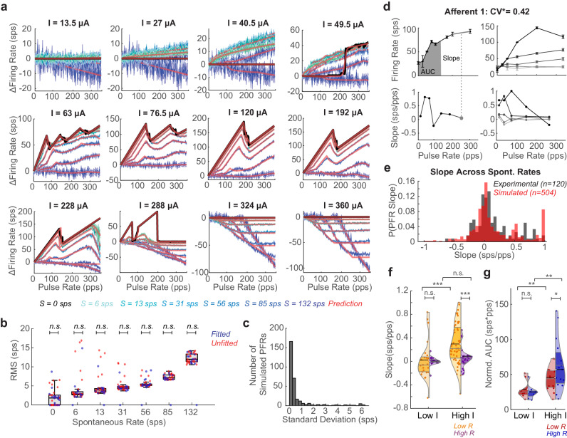
Fig. 4. Testing prediction equations against data.
a Fit of the equations (red) to PFR of vestibular afferents of different spontaneous rates (colored like to dark blue as S increases. S = 0 in black. Data plotted as mean ± SEM across simulations. b RMS between prediction and simulation for afferent models (N = 10) of each spontaneous rate. PFRs where parameters were fit directly (blue) and interpolated between the fitted parameters (red). Unpaired t-test showing no significant difference between the two (n.s.). Exact values in Supplementary Table 2. Minimum, maximum, and median (center) across amplitudes shown. c RMS per PFR across all simulations with different random seeds. d Experimental recordings from Afferent 1 (left). PFR at single I with slope highlighted on PFR and corresponding slope on pulse rate-slope plot (gray dot). AUC of firing rate at low R (R < 150 pps) also shown (gray fill). (right) PFR and pulse rate-slope plot at increasing Is for the same afferent. Data are plotted as mean ± SEM across simulations. e PDF comparison of experimental slopes (collected as in d, black) to slopes of simulated afferents sampled every 30 pps at seven current steps between 18 and 312 μA (red). f Violin plots of distribution of slopes at low R (orange) versus high R (R > 150 pps, purple) for stimulation with high Is (I > 0.5Imax) versus low Is per afferent. At low I, slopes are not significantly different between low R(N = 23) and high R(N = 17) (t(38) = 0.237, p = 0.81). At high I, slopes are significantly different between low R(N = 54) and high R(N = 26)(t(78) = 3.32, p = 0.0014). Mean marked with black line and color-matched semicircle. Median and quartiles marked with gray lines. At low versus high I, slopes at low R are significantly different but not at high R (t(75) = 3.23, p = 0.0028; t(41) = 1.19, p = 0.24). g Violin plots of normalized AUC in low R and high R section of the PFR for stimulation at low I(red) and high I(blue). At low I(N = 8), AUCs in the low and high R region of the PFR are not significantly different, but at high I(N = 15) the AUCs are significantly different (t(14) = 0.654, p = 0.523; t(28) = 1.79, p = 0.0083). All the significances reported are for two-tailed t-tests. Significance in f-g is shown as *p < 0.1;**p < 0.05;***p < 0.01 (Supplementary Table 3).

