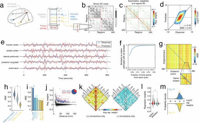
Fig. 1. Fitting and characterizing weighted, signed, and asymmetric structural connectivity.
a Here, we used linear model to estimate regression (edge) weights. For a given region i, we identified its structurally connected neighbors and used their past activity to predict node i's future activity. This procedure results in a series of regression weights; one weight is associated with each neighbor. b Those weights were then entered into the binary structural connectivity “mask''. When this procedure was repeated for all i ∈ [1, …, n] it generates a weighted, signed, and asymmetric matrix whose nonzero entries are masked by structural connections (see panel c). d Two-dimensional histogram showing observed and predicted activity, pooled across all participants and scans. Colors indicate number of samples in any bin. e Examples of observed and predicted activity for five select regions in a single subject and scan. f Similarity of regression weights (edge weights) as a function of amount of data. Note that units on x-axis are expressed as fraction of time points in scan, where the total number of frames was 1099. g Weights fit using scans from subject s are better at predicting activity in held-out scans from s than other subjects, . In this figure, the blocks along the diagonal are 4 × 4 and represent the four resting-state HCP scans. h Distributions of errors in model fit, grouped by whether the model is being used to predict activity in a scan of a different subject (N = 142880), the held-out scan from the same subject (N = 1140), or one of the scans used in fitting the weights (N = 380). i Comparison of model errors using the observed network with a minimally wired network, one in which rows/columns were randomly reordered, and another in which time series were circularly shifted (independently across regions, scans, and subjects). j Relationship of regression weights and Euclidean distance. We also identified edges whose regression weights were much stronger than expected (those above the dashed line). k Distribution of regression weights across canonical brain systems (Cont = Control, DMN = default mode network, DAN = dorsal attention network, Lim = limbic, Sal/VAN = salience, SMN = somatomotor, TP = temporoparietal, Vis = visual). l Comparison of within- (N = 4654) and between-system (N = 24,370) regression weights. All box plots, shown in red and overlaid on data points in e and f, depict the interquartile range (IQR) and the median value of the distribution. Whiskers extend to the nearest points ± 1.5 × IQR above and below the 25th and 75th percentiles. Asterisks indicate a significant difference between box plots. m Comparison of positive and negative weights.

