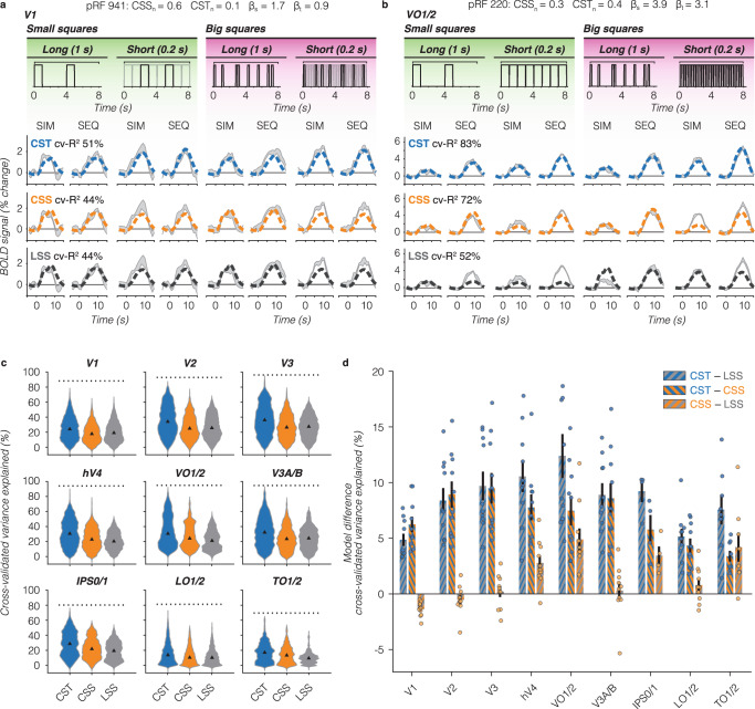
Fig. 6. Comparison of performance across pRF models.

a V1 example voxel time series. Gray shaded area: average ± SEM across repeats for each stimulus condition. Data are from the same voxel as in Fig. 2a repeated for each row. PRF model fits are shown in dashed lines. Split-half cross-validated variance explained (cv-R²) is computed by fitting the predicted time series to the average of odd runs and applying the model fit to the average of even runs and vice versa. Blue: CST summation model (top row). Orange: CSS model (middle row). Black: LSS model (bottom row). b VO1/2 example voxel. Data are from the same voxel as in Fig. 3a repeated for each row. Same color scheme as panel A. c Distribution of voxel-level cv-R² for each pRF model, all ten participants. Triangle: median. Dotted line: noise ceiling computed from max split-half reliability across participants. Blue: CST. Orange: CSS. Gray: LSS. Since a number of voxels varies per participant and visual area, we assure equal contribution of each participant by resampling data 1000 times of each participant’s visual area. d Pairwise model comparison for each visual area. Bars: average across ten participants of the voxelwise difference in cv-R² between two pRF models. Error bars: SEM across ten participants. Individual dots: average difference for each participant. Blue-gray: CST vs LSS. Blue-orange: CST vs CSS. Orange-gray: CSS vs LSS.