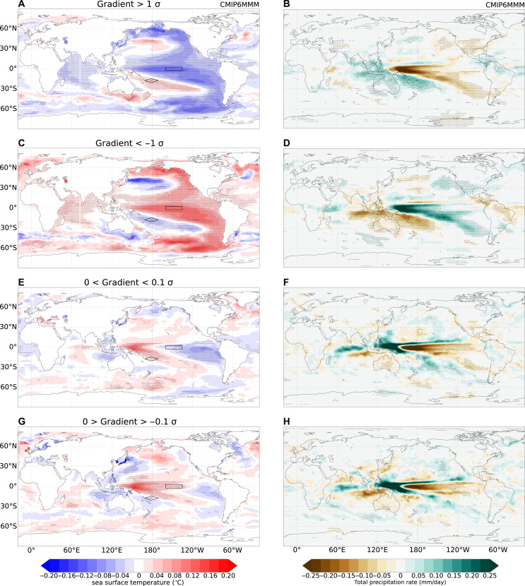
Fig. 4. Composite maps of simulated SST (left) and precipitation (right).

(A to H) In each case, four different regimes are included based on the magnitude of the SWCP gradient calculated using data from 16,062 years of the CMIP6 preindustrial control simulation. (A) and (B) represent composites obtained when there is a strong positive SWCP gradient (i.e., warmer temperature over Fiji compared to central Pacific and the magnitude of the gradient is >1 SD), and (C) and (D) represent a strong inverse SWCP gradient (i.e., warmer temperature in the central Pacific than in Fiji and the SWCP gradient is <−1 SD). The bottom two rows represent composites when the SWCP gradient is weaker (less than 0.1 SD), with (E) and (F) showing composite maps when the gradient is weak and positive and (G) and (H) representing composites when the gradient is weak and negative. Stripling on the plots represents significant values at 95% significance level using a two-tailed t test. Composites from each model are computed first before calculating the MMM composite to provide equal weightage to each CMIP6 model used in the study.