The decoder design and performance comparative analysis for closed-loop brain–machine interface system

Abstract

Brain–machine interface (BMI) can convert electroencephalography signals (EEGs) into the control instructions of external devices, and the key of control performance is the accuracy and efficiency of decoder. However, the performance of different decoders obtaining control instructions from complex and variable EEG signals is very different and irregular in the different neural information transfer model. Aiming at this problem, the off-line and on-line performance of eight decoders based on the improved single-joint information transmission (SJIT) model is compared and analyzed in this paper, which can provide a theoretical guidance for decoder design. Firstly, in order to avoid the different types of neural activities in the decoding process on the decoder performance, eight decoders based on the improved SJIT model are designed. And then the off-line decoding performance of these decoders is tested and compared. Secondly, a closed-loop BMI system which combining by the designed decoder and the random forest encoder based on the improved SJIT model is constructed. Finally, based on the constructed closed-loop BMI system, the on-line decoding performance of decoders is compared and analyzed. The results show that the LSTM-based decoder has better on-line decoding performance than others in the improved SJIT model.

Introduction

Brain–machine interface (BMI) can convert the collected electroencephalography signals (EEGs) into corresponding instructions to control external devices, so as to realize the interaction between the brain and outside world (Lebedev and Nicolelis 2006; Romero-Laiseca et al. 2020; Pan et al. 2022). The structure of closed-loop BMI system is shown in Fig. 1, which is consist of the decoder, encoder and external device. The decoder and encoder are both the mathematical model essentially (Xiao et al. 2019; Pan et al. 2022). The decoder is used to extract motion intention related to the task, and convert it into corresponding instructions to control the motion of external devices; the encoder is used to feed back motion-related perception and state information to the brain (Pan et al. 2020, 2021).

Fig. 1.

The structure of closed-loop BMI system

It can be seen from the Fig. 1 that the decoder converts EEG signals into brain command to directly act on external devices, and repeatedly affects the system performance in the closed-loop control process (Orset et al. 2020; Pan et al. 2021). Although many studies have confirmed that the BMI closed-loop system including the encoder has better control effectiveness than the open-loop BMI system only including the decoder, in some application scenarios, the feedback of the closed-loop BMI system is difficult to produce effective influence due to the change of actual neural activity (Pan et al. 2022). Therefore, the decoder plays an pivotal role in the whole BMI system, and its decoding performance directly affects the control effectiveness of the BMI system on external devices. So it is of great significance to design a decoder with superior decoding performance. The decoders have based on the variety of principles have been designed, which are mainly divided into: machine learning methods based on mathematical statistics, deep learning methods based on artificial neural networks (ANN) and decoding methods based on filters (Nakagome et al. 2020; Shanechi 2017; Dethier et al. 2013).

The machine learning method based on mathematical statistics is decoding and analyzing data by constructing a statistical model of data probability, and classical principles mainly include the following. Multivariate non-linear regression (MNLR) determines the qualitative relationship between variables by using regression analysis (Robinson et al. 2013). Its advantage is that it can more accurately fit the non-linear relationship between multiple independent variables and dependent variables. However, its modeling is difficult, and the convergence depends too much on the selection of initial values. Therefore, when the data is complex, MNLR cannot describe a specific expression well (add ref) (Zhang et al. 2018). K-nearest neighbor (KNN) is a nonparametric, non-linear classifier. It uses the distance between the sample point to classify data, which avoids the problem of unknown function well (Yu et al. 2016; Bablani et al. 2018). Benefiting from the advantages of simple principle, easy implementation and no need to estimate parameters, KNN-based decoders can be used to solve multimodal problems. However, KNN-based decoder is highly sensitive to the data dimension, and its computational complexity increases rapidly with the increase of the data dimension. In addition, KNN-based decoders overly rely on the selection of EEGs feature vectors. Mousa et al. (2016), Makin et al. (2020). Similar principles also include support vector regression (SVR), and SVR-based decoder can achieve good accuracy without a large amount of training data (Dong et al. 2017; Varsehi and Firoozabadi 2021). In different, SVR project the feature vectors into another high-dimensional space, so it has more unique advantages in solving high-latitude, multi-pattern and non-linear recognition. However, it is also limited to small sample data (Yan et al. 2012). Random forest (RF) decodes data by integrating multiple decision trees, and the training data of each decision tree is obtained by independent sampling. RF-based decoder solves the problems of accuracy and computational efficiency when the sample data is large, and it can handle non-linear and multi-pattern recognition well. However, RF is more susceptible to sample data quality and prone to overfitting in noisy situations (Balamurugan et al. 2020; Shi et al. 2022). Partial Least Squares (PLS)is a mathematical optimization technique that finds the best functional match for a set of data by minimizing the sum of squares of errors (Foodeh et al. 2020). It can perform regression modeling under the condition that the independent variables have serious multiple correlations, and also allows regression modeling under the condition that the number of sample points is less than the number of variables (Ahmadi et al. 2020). However, PLS regression method requires a sufficient number of independent variables to ensure the selection of its components. In addition, the regression coefficients of PLS are less interpretable (Chu et al. 2020; Chao et al. 2010).

As an empirical method based on performance optimization, ANN can decode and judge data without any analytical equation and system description (Soures and Kudithipudi 2019; Zou and Cheng 2021; Cheng et al. 2019; Huang et al. 2019), and can approximate the continuous function with arbitrary accuracy, especially for the non-linear function. Moreover, ANN avoids the deficiencies of plane radial flow of mathematical statistics, and has good non-linear mapping capabilities. As a classic ANN, back propagation (BP) neural network is a multilayer feedforward network trained by error back propagation. It can adjust the weights of each unit to fit the non-linear mapping relationship, and is very suitable for solving high-latitude problems with complex internal mechanisms. However, BP algorithm is a fast gradient descent algorithm, it is easy to fall into the problem of local minimum, and it does not have memory function (Di and Wu 2015; Jin and Zhang 2013). In order to realize the function of long-term learning and storing information, Long short-term memory (LSTM) network was proposed by improving the gradient of recurrent neural network. It realizes the functions of forgetting and memory by using a structure through which information is selectively passed, and has outstanding performance on time sequential data (Nakagome et al. 2020; Sun et al. 2019). However, the structure of the LSTM model is relatively complex, and the training takes a long time (Wang et al. 2018). Although ANN avoids the deficiencies of mathematical statistics and has the advantages of associative memory function and nonlinear mapping, due to its strong nonlinear fitting ability, choosing a decoder based on neural network will cause problems such as long learning time, over fitting, large training data volume and complex network parameter setting (Zhang et al. 2019; Lotte et al. 2018).

The filters is to optimally estimate data with considering noise, so it can well avoid the problems of poor data quality (Li et al. 2009). Wiener filter (WF) is a linear filter based on the criterion of minimum mean squared error. It can obtain an optimal estimation by carrying out overall estimation of data and has global optimality. In addition, it has strong adaptability and can handle noisy EEGs well. However, it is needed to deduce all past values, and the autocorrelation and cross-correlation function need to be updated for each new data, resulting in low computational efficiency (Pan et al. 2020; Kobler et al. 2020). Kalman filter (KF) is a recursive estimation filter, mainly solving linear problems by means of conditional expectations and state transitions. The values of adjacent data is only needed in the recursive process, which solves the problem of computational efficiency in WF well. However, KF has a weaker memory function than WF, and is limited on the assumption of linearity (Li et al. 2014; Pan et al. 2016; Gamal et al. 2021). Extended Kalman filter (EKF) replaces the state transition and observation functions in KF with differentiable and non-linear functions, so that it can adapt to non-linear data, but it still relies on Gaussian distribution conditions (Yu et al. 2016).

To sum up, different principles have unique advantages and disadvantages. Machine learning methods can analyze the probability distribution of data, and have good generalization, but their solution needs complex analysis of system (Nakagome et al. 2020; Yan et al. 2012). As a data-driven classification method, the ANN features associative memory and nonlinear mapping. Therefore, in the case of sufficient data, the ANN based decoder has better decoding effectiveness. However, it has the problem of over-fitting, and is greatly affected by the quality of data (Soures and Kudithipudi 2019; Gamal et al. 2021). The decoding methods based on filters avoid the influence of poor data quality, but its non-linear mapping and memory function is not as good as the ANN (Li et al. 2009). Therefore, for the design of decoder, it is necessary to compare the performance of the classic principles among three types of methods.

In this paper, a variety of decoder structures based on the improved single-joint information transmission (SJIT) model are designed to decode the control instructions of the human brain to external devices in the closed-loop BMI system. Specifically, 9 decoders based on the improved SJIT model are designed and the off-line decoding performance of them are tested. Then, the RF-based encoder and the designed decoder are used to construct a closed-loop BMI system based on the improved SJIT model. Finally, we compare the online decoding performance of different decoders and analyze the reasons for the performance differences of different decoders. Our main contributions can be summarized as follows.

1. We design a variety of classical decoder architectures based on the improved SJIT model and quantitatively compare and analyze the off-line performance of different decoders;

2. We build a closed-loop BMI system based on the improved SJIT model by combining the encoder based on random forest and the decoder designed. So that different decoders can compare their decoding capabilities of EEGs under the same neural information transmission model;

3. The quantitative and qualitative analysis demonstrate that the decoder based on LSTM method has the best decoding effectiveness in the closed-loop BMI system based on the improved SJIT model.

Improved SJIT model

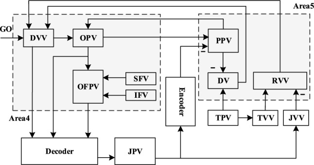
Pan et. al proposed the improved SJIT model on the basis of the literature (Bullock et al. 1998), the model shows the essential cortical pathways of information transmission for voluntary single-joint movement, as shown in Fig. 2, it includes the brain areas 4 and 5 (Pan et al. 2020).

Fig. 2.

The structure of improved SJIT model

The related abbreviations and their designation in this model are shown in Table 1.

Table 1.

Neurons designation and abbreviation in improved SJIT model

Designation	Abbreviation	Designation	Abbreviation
Desired velocity vector	DVV	Joint velocity vector	JVV
Outflow position vector	OPV	Relative velocity vector	RVV
Target velocity vetctor	TVV	Joint position vector	JPV
Static force vector	SFV	Dynamic gamma motoneurons	${\gamma }^d$
Inertial force vector	IFV	Static gamma motoneurons	${\gamma }^s$
Perceived position vector	PPV	Alpha motoneuron	$\alpha$
Difference vector	DV	Type Ia afferent fibers	Ia
Target position vector	TPV	Type II afferent fibers	II
Outflow force and position vector	OFPV

The “DV” neurons is used to calculate the difference between the perceived and the target joint position. The firing activity $r_i(t)$ of “DV” neurons can be described as:

$$\begin{array}{c}\hfill r_i(t)=max\{T_i(t)-x_i(t)+B^r,0\}\end{array}$$ 1

where t is continuous time; $T_i(t)$ and $x_i(t)$ are the average firing activity of “TPV” and “PPV” neurons, and they can continuously calculate current position of agonist muscle; the subscript i indicates that the firing activity corresponds to agonist muscle, and is the same through out the subsequent introduction; $B^r$ represents the base firing activity of “DV” neurons.

The output $v_i^T(t)$ and $v_i^P(t)$ corresponding to “TVV” and “JVV” neurons can be described as:

$$\begin{array}{c}\hfill v_i^T(t)=\frac{\text{d}{T}_i(t)}{\text{d}t},v_i^P(t)=\frac{\text{d}{p}_i(t)}{\text{d}t}\end{array}$$ 2

where $p_i$ represents the average firing activity of “JPV” neurons. The “RVV” neurons are used to describe the relative velocity between the “TPV” and “JPV” neurons, and its output $v_i^R$ can be expressed as:

$$\begin{array}{c}\hfill v_i^R(t)=v_i^T(t)-v_i^P(t)\end{array}$$ 3

The calculated $r_i(t)$ is transmitted to the “DVV” neurons, and then the average firing activity $u_i(t)$ of “DVV” neurons is obtained after scaling up and down:

$$u_i(t)=max\left[g(t)\left(r_i(t)-r_j(t)+\zeta \left(v_i^R(t)-v_j^R(t)\right)\right)+B^u,0\right]$$ 4

where $B^u$ is the base firing activity of “DVV” neurons; g(t) represents the “GO” signal in Fig. 2, is the scaling factor of “DVV” and generated from the basal ganglia, which can control the magnitude of “DVV” without altering the direction; $\zeta$ is the compensation coefficient of “RVV” neurons; and the subscript j indicates that the firing activity corresponds to the antagonistic muscle, which will be the same in the following introduction.

The “GO” signal does not change suddenly, and its dynamic form can be represented with a two-step cellular cascade:

$$\begin{array}{cc}\hfill \frac{\text{d}{g}^1(t)}{\text{d}t}& =ϵ\left(-,g^1,(t),+,(C-g^1(t)),g^0\right)\hfill \end{array}$$ 5a

$$\begin{array}{cc}\hfill \frac{\text{d}{g}^2(t)}{\text{d}t}& =ϵ\left(-,g^2,(t),+,(C-g^2(t)),g^1,(t)\right)\hfill \end{array}$$ 5b

$$\begin{array}{cc}\hfill g(t)& =g^0\frac{g^2(t)}{C}\hfill \end{array}$$ 5c

where $ϵ$ is a constant that represents slow integration rate; C is the saturation value; and $g^0$ is a constant from the forebrain decision center, which can determine the magnitude of “GO” signal.

The “OPV” neurons are related to tonic neurons and shows the outflow position. The firing activity of “OPV” neurons can be described as:

$$\begin{array}{cc}\hfill \frac{\text{d}{y}_i(t)}{\text{d}t}& =(1-y_i(t))(\eta x_i(t)+max\{u_i(t)-u_j(t),0\})\hfill \\ \hfill & -y_i(t)(\eta x_j(t)+max\{u_j(t)-u_i(t),0\})\hfill \end{array}$$ 6

where $\rho$ is the scaling factor. Static (${\gamma }_i^S(t)$) and dynamic (${\gamma }_i^D(t)$) gamma motoneurons are used to transmit the commands from the brain to joints. The firing activity of these motoneurons can be described as:

$$\begin{array}{cc}\hfill {\gamma }_i^S(t)& =y_i(t)\hfill \end{array}$$ 7a

$$\begin{array}{cc}\hfill {\gamma }_i^D(t)& =\rho max\{u_i(t)-u_j(t),0\}\hfill \end{array}$$ 7b

where $\rho$ is the scaling factor.

The primary (“Ia”) and secondary (“II”) muscle spindle afferents are used to transmit the information of joint position to the “PPV” neurons, and their firing activity $s_i^1(t)$, $s_i^2(t)$ can be modeled as:

$$\begin{array}{cc}\hfill s_i^1(t)& =S\left(\theta ,max,\left\{{\gamma }_i^S,(t),-,p_i,(t),,,0\right\}\right)\hfill \\ \hfill & \left(+,\varphi ,max,\left\{{\gamma }_i^D,(t),-,\frac{\text{d}{p}_i(t)}{\text{d}t},,,0\right\}\right)\hfill \end{array}$$ 8a

$$\begin{array}{cc}\hfill s_i^2(t)& =S\left(\theta ,max,\left\{{\gamma }_i^S,(t),-,p_i,(t),,,0\right\}\right)\hfill \end{array}$$ 8b

where $\theta$ represents the sensitivity of nuclear chain fibres and the static nuclear bag fibres; $\varphi$ represents the sensitivity of dynamic nuclear bag fibres; and the function of afferent fiber activity S can be calculated by $S(\omega )=\omega /(1+100{\omega }^2)$. The firing activity $x_i(t)$ of “PPV” neurons can be described as:

$$\begin{array}{cc}\hfill \frac{\text{d}{x}_i(t)}{\text{d}t}& =(1-x_i(t))max\left\{\varrho ,y_i,(t),,+,,s_j^1,(t-\tau ),,-,,s_i^1,(t-\tau ),,,0\right\}\hfill \\ \hfill & -x_i(t)max\left\{\varrho ,y_j,(t),,+,,s_i^1,(t-\tau ),,-,,s_j^1,(t-\tau ),,,0\right\}\hfill \end{array}$$ 9

where $\tau$ represents the delay time of spindle feedback; and $\varrho$ represents the constant gain, and $s_i^1(t-\tau )-s_j^1(t-\tau )$ is the feedback position vector of “Ia” muscle spindle afferents, and denoted as $s^1(t)$. The firing activity of the “IFV” and “SFV” neurons can be described as:

$$\begin{array}{cc}\hfill q_i(t)& ={\lambda }_{i}max\left\{s_i^1,(t-\tau ),-,s_i^2,(t-\tau ),-,\mathrm{\Lambda },,,0\right\}\hfill \end{array}$$ 10

$$\begin{array}{cc}\hfill \frac{\text{d}{f}_i(t)}{\text{d}t}& =(1-f_i(t))h{s}_i^1(t-\tau )\hfill \\ \hfill & -\psi f_i(t)\left(f_j,(t),+,s_j^1,(t-\tau )\right)\hfill \end{array}$$ 11

where $q_i(t)$ and $f_i(t)$ are the average firing activities of the “IFV” and “SFV” neurons; $\mathrm{\Lambda }$ represents a constant threshold; h is the constant gain, and controls the velocity and strength of the external load compensation; and $\psi$ is the inhibitory scaling parameter. The “OFPV” neurons are used to provide the phasic-tonic activity, and the firing activity $a_i(t)$ of “OFPV” neurons can be represented as:

$$\begin{array}{c}\hfill a_i(t)=y_i(t)+q_i(t)+f_i(t)\end{array}$$ 12

The firing activity ${\alpha }_i(t)$ of alpha motoneurons can be modeled as:

$$\begin{array}{c}\hfill {\alpha }_i(t)=a_i(t)+\delta s_i^1(t)\end{array}$$ 13

where $\delta$ represents the stretch reflex gain.

Based on the above firing activity, the joint dynamics can be described as:

$$\begin{array}{c}\hfill \frac{{\text{d}}^2{p}_i(t)}{\text{d}{t}^2}=\frac{1}{I}\left(\mathrm{\Delta },M,+,E_i,-,V,\frac{\text{d}{p}_i(t)}{\text{d}t}\right)\end{array}$$ 14

where $p_i(t)$ is always located between origin-to-insertion distances of agonist muscle motion, and $p_i(t)+p_j(t)=1$; I represents the rotational inertia; V represents the viscosity; $E_i$ represents the external force imposed on the joint; $\mathrm{\Delta }M$ is the total force generated by muscles, and $\mathrm{\Delta }M=M(c_i(t)-p_i(t))-M(c_j(t)-p_j(t))$; $M(c_i(t),p_i(t))$ is the force generated by agonist muscle, and $M(c_i(t),p_i(t))=max\{c_i(t)-p_i(t),0\}$; $c_i(t)$ represents the activity of muscle contraction and can be described as:

$$\begin{array}{c}\hfill \frac{\text{d}{c}_i(t)}{\text{d}t}=\nu (-c_i(t)+{\alpha }_i(t))\end{array}$$ 15

where $\nu$ is the contraction rate of muscles. Note: visual feedback is not considered in this model. In the simulation in this paper, the position $p_i(t)$ of agonist muscle is used to represent the position $P_i(t)$ of joint.

Design and off-line test of decoders

For healthy people, the body has a complete brain information transmission pathway. As shown in Fig. 2, the firing activity of “DVV”, “OPV” and “OFPV” neurons can be transmitted to the muscles through the spinal cord circuit for controlling limb motion. However, for the disabled with spinal cord injury, they cannot complete the above-mentioned brain information transmission, and the decoder can convert EEGs into control instructions of muscles or external devices, so the decoder can provide assistance for the disabled. In addition, since the accuracy of decoders affects the control accuracy, designing a decoder with superior decoding performance is very critical for the entire BMI system (Kumar et al. 2013). The design of decoders based on MNLR, KNN, SVR, RF, BP neural network, LSTM network, WF, KF and PLS are mainly introduced in this section.

MNLR-based decoder

Assuming that the relationship between the firing activities of neurons and the total force $\mathrm{\Delta }M(k)$ is a non-linear function, and the MNLR model is established as follows:

$$\begin{array}{c}\hfill \mathrm{\Delta }\overline{M}(k)={\left(\sum _{h=1}^H,{\xi }_h,z_h,(k),+,{\xi }_0\right)}^3\end{array}$$ 16

where $z_h(k)$ represents the average firing activities of the h-th neuron at time k (k-th set of training data); $z_1(k),z_2(k),\dots ,z_6(k)$ correspond to the average firing rate $a_i(k),a_j(k),u_i(k),u_j(k),y_i(k),y_j(k)$, H corresponds to the number of neurons, and $H=6$; ${\xi }_h$ and ${\xi }_0$ are the weights. $\mathrm{\Delta }\overline{M}(k)$ is the output of the decoder in the improved SJIT model.

The non-linear least squares algorithm (Levenberg–Marquardt algorithm) is used to find the parameter $[{\xi }_0,{\xi }_1,{\xi }_2,\dots ,{\xi }_H]$ that minimizes the formula (17):

$$\begin{array}{c}\hfill minQ({\xi }_0,{\xi }_1,\dots ,{\xi }_H)=\sum _{k=1}^N{(\mathrm{\Delta }\overline{M}(k)-\mathrm{\Delta }M(k))}^2\end{array}$$ 17

where N is the number of sample data; $\mathrm{\Delta }M(k)$ is the output of the Spinal Cord Circuit in the improved SJIT model (target value).

KNN-based decoder

The main idea of KNN is to calculate the difference between the current data and training data, and then selects the K sets of training data with the smallest difference to decode the $\mathrm{\Delta }M(k)$ (Varsehi and Firoozabadi 2021). Euclidean distance is used to measure the difference between the current data and training data, as shown in (18):

$$\begin{array}{c}\hfill S(k)=\sqrt{\sum _{h=1}^H{(z_h(k)-{\overline{z}}_h(i))}^2}i=1,2,\dots ,I\end{array}$$ 18

where ${\overline{z}}_h(i)$ represents the average firing activities of h-th neuron in i-th set of training data; $z_h(k)$ represents the average firing activities of h-th neuron in k-th set of test data; S(k) is the Euclidean distance between the k-th set of test data and i-th set of training data; and I is the number of training samples.(problem!)

The K sets of training data with the smallest Euclidean distance are selected, the Euclide distances between the current test data $z_h(k)$ and these K sets of training data are denoted as $S_l$, their corresponding total force as $\mathrm{\Delta }{M}_l$, and $l=1,2,\dots K$. The decoding output $\mathrm{\Delta }\overline{M}(k)$ of the model about test data ${\overline{z}}_h(k)$ is represented as:

$$\begin{array}{cc}\hfill \mathrm{\Delta }\overline{M}(k)& =\sum _{l=1}^K{\beta }_l\mathrm{\Delta }{M}_l\hfill \end{array}$$ 19

$$\begin{array}{cc}\hfill {\beta }_l& =\frac{S_l^{-1}}{{\sum }_{l=1}^K{S}_l^{-1}}\hfill \end{array}$$ 20

where ${\beta }_l$ is the weight corresponding to $\mathrm{\Delta }{M}_l$.

SVR-based decoder

SVR is derived from support vector machines, which decodes data by finding a regression model that minimizes the deviation between the regression value and target value (Roy et al. 2019). Specific as follows: training data as $(\mathbf{z}(1),\mathrm{\Delta }M(1))$, $(\mathbf{z}(2),\mathrm{\Delta }M(2)),\dots ,(\mathbf{z}(N),\mathrm{\Delta }M(N))$, $\mathbf{z}\in R^H$, $\mathrm{\Delta }M\in R$, R represents the real number. Assuming there is a regression model, which can make $\mathrm{\Delta }\overline{M}(k)$ and $\mathrm{\Delta }M(k)$ infinitely similar, as follows:

$$\begin{array}{c}\hfill \mathrm{\Delta }\overline{M}(k)=W_s\ast \mathbf{z}(k)+b_s\end{array}$$ 21

where $W_s$ and $b_s$ are the weight and bias coefficients of regression model.

The solution of SVR can be transformed into an optimization problem. In order to prevent over-fitting the training samples, the optimization calculation will be not carried out when the deviation between $\mathrm{\Delta }\overline{M}(k)$ and $\mathrm{\Delta }M(k)$ is less than $\vartheta$, as shown below:

$$\begin{array}{c}\hfill min\frac{1}{2}||W_s{||}^2+B\sum _n^N{l}_{\vartheta }(\mathrm{\Delta }M(k),\mathrm{\Delta }\overline{M}(k))\end{array}$$ 22

where B is the penalty factor; $\vartheta$ is the tolerable deviation; the function $l_{\vartheta }$ is the insensitive loss function of $\vartheta$, and its calculation is as follows:

$$_{\vartheta }^{}(\mathrm{\Delta }M,\mathrm{\Delta }\overline{M})=\left\{\begin{array}{cc}0,\hfill & \text{if}|\mathrm{\Delta }M(k)-\mathrm{\Delta }\overline{M}(k)|<\vartheta \\ |\mathrm{\Delta }M(k)-\mathrm{\Delta }\overline{M}(k)|-\vartheta ,\hfill & \text{otherwise}\end{array}\right)$$ 23

In order to make all the data fit the regression model, the relaxation factor is introduced, $\chi (k)$ and ${\chi }^{\ast }(k)$ represent the upper and lower bounds of relaxation factors, and $\chi (k),{\chi }^{\ast }(k)\ge 0$, and then the constraint $|\mathrm{\Delta }M(k)-\mathrm{\Delta }\overline{M}(k)|<\vartheta$ becomes:

$$\begin{array}{c}\hfill \left\{\begin{array}{cc}& \mathrm{\Delta }M(k)-\mathrm{\Delta }\overline{M}(k)<\vartheta +\chi (k)\hfill \\ \hfill & \mathrm{\Delta }\overline{M}(k)-\mathrm{\Delta }M(k)<\vartheta +{\chi }^{\ast }(k)\hfill \\ \hfill \end{array}\right)\end{array}$$ 24

After introducing the relaxation factor, the optimization of SVR can be expressed as solving the $W_s$ and $b_s$ that minimizes $\mathrm{{\rm Y}}$, as follows:

$$\begin{array}{c}\hfill \left\{\begin{array}{c}min\mathrm{{\rm Y}}=\frac{1}{2}||W_s{||}^2+B{\sum }_k^N(\chi (k)+{\chi }^{\ast }(k))\hfill \\ \text{s.t.}{W}_s\ast \mathbf{z}(k)+b_s-\mathrm{\Delta }\overline{M}(k)<\vartheta +\chi (k)\hfill \\ \mathrm{\Delta }\overline{M}(k)-W_s\ast \mathbf{z}(k)-b_s<\vartheta +{\chi }^{\ast }(k)\hfill \end{array}\right)\end{array}$$ 25

The Lagrange optimization algorithm is used to transform it into a dual problem for solving the optimal parameters $W_s$ and $b_s$, and then the output of the decoder $\mathrm{\Delta }\overline{M}$ can be calculated by (30a).

RF-based decoder

RF uses the bootsrap resampling to extract multiple samples from training data, and establishes a decision tree on the sampled set each time, and then conducts a model by combining multiple decision trees (Seraj and Sameni 2017). By establishing different decision tree on the random sampled set, the difference of decision tree models can be increased, and then the decoding ability will be improved.

The details are as follows: through J rounds of sampling, the $\varsigma$-th decision tree $d(\mathbf{z}(k),Q_{\varsigma })$ is obtained, $\varsigma =1,2,\dots ,J$, and $Q_{\varsigma }$ corresponds to the target output ($\mathrm{\Delta }{M}_{\varsigma }$) of the sampled data, and then a decision tree model is constructed by combining them. Given the independent variable z(k) at the current time, each decision tree will have an output $\mathrm{\Delta }{M}_{\varsigma }(k)$. Here, the mean value of the output results of all decision trees is used as the combined model output, as shown below:

$$\begin{array}{c}\hfill \mathrm{\Delta }\overline{M}(k)=\frac{1}{J}\sum _{\varsigma =1}^{J}d(\mathbf{z}(k),Q_{\varsigma })\varsigma =1,2,\dots ,J\end{array}$$ 26

BP-based decoder

ANN is an information processing method developed by imitating the function and structure of the biological nervous system, among which BP neural network is a multi-layer feed-forward network with error back propagation (Yan et al. 2020). BP neural network is composed of three parts: input layer, hidden layer and output layer, as shown in Fig. 3.

Fig. 3.

The structure diagram of BP neural network

In the forward propagation, that is, the process of data from the input layer to the output layer, $z_{\mu }(k)$ as the output of the $\mu$-th neuron in the first hidden layer of BP neural network can be expressed as:

$$\begin{array}{c}\hfill z_{\mu }(k)=\sum _{h=1}^H{w}_{h,\mu }{z}_h(k)\end{array}$$ 27

where $z_h(k)$ is the input of BP neural network; $w_{h,\mu }$ is the weight connecting the input layer and hidden layer; H is the number of neurons in the input layer of BP neural network (i.e., the number of neurons mentioned above). The output of hidden layer ${\acute{z}}_{\mu }(k)$ can be expressed as:

$$\begin{array}{c}\hfill {\acute{z}}_{\mu }(k)=f(z_{\mu }(k))=\frac{1}{1+e^{-z_{\mu }(k)}}\end{array}$$ 28

Starting from the second hidden layer, the output of neurons in the upper layer is taken as the input of neurons in the current layer, and the calculation is similar to that of the first layer. The output of neurons in the output layer can be expressed as:

$$\begin{array}{c}\hfill \mathrm{\Delta }\overline{M}(k)=\sum _{\mu }^{H_1}{w}_{o,\mu }{\acute{z}}_{\mu }(k)\end{array}$$ 29

where $w_{o,\mu }$ is the weight connecting the $\mu$-th neuron in the last hidden layer and neuron in output layer; $H_1$ represents the number of neurons in the last hidden layer. The error of BP neural network can be expressed as (30a), and the error index function as (30b):

$$\begin{array}{cc}\hfill e(k)& =\mathrm{\Delta }M(k)-\mathrm{\Delta }\overline{M}(k)\hfill \end{array}$$ 30a

$$\begin{array}{cc}\hfill E& =\frac{1}{2}{[e(k)]}^2\hfill \end{array}$$ 30b

During back propagation, the Levenberg–Marquardt algorithm is used to adjust the weights, and the weight change connecting the output layer and hidden layer $\mathrm{\Delta }{w}_{o,\mu }$ can be calculated as:

$$\begin{array}{c}\hfill \mathrm{\Delta }{w}_{o,\mu }=-\kappa \frac{\partial E}{\partial w_{o,\mu }}\end{array}$$ 31

where $\kappa$ is the learning rate of BP neural network. The weight of iteration at the next time becomes:

$$\begin{array}{c}\hfill w_{o,\mu }(k+1)=w_{o,\mu }(k)+\mathrm{\Delta }{w}_{o,\mu }\end{array}$$ 32

The calculation of the weights $w_{h,\mu }$ from the input layer to the hidden and between hidden layers is similar to that of $w_{o,\mu }$.

LSTM-based decoder

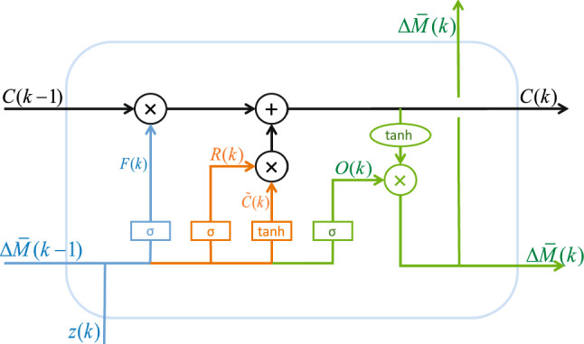
The LSTM network was proposed by Hochreiter S and Schmidhuber J in 1997 to solve the problem of long-distance dependence in RNN (Tseng et al. 2019). Three gates are added to the cell unit of RNN network, namely forget gate, input gate and output gate, and its structure diagram is shown in Fig. 4. The forget gate is used to control the preservation of the historical state information of cell unit, and the activation function $\sigma$ makes the output value of the forget gate between [0, 1]. When the forgetting gate output is closer to 1, it means that the previous state information is retained more. The input gate is used to control the input of information and determine how much will be added to the memory. The output gate is used to control the output of information and determine how much memory information is used in the next update stage.

Fig. 4.

The structure diagram of LSTM network

The specific is as follows: the first step is to determine the information to enter cell unit, shown the part blue in Fig. 4, the formula is as follows:

$$\begin{array}{c}\hfill F(k)=\sigma (W_f\ast [\mathrm{\Delta }\overline{M}(k-1),\mathbf{z}(k)]+b_f)\end{array}$$ 33

where F(k) is the output of forget gate; $W_f$ is the weight matrix; $b_f$ is the bias vector of forget gate; $\mathrm{\Delta }\overline{M}(k-1)$ represents the output at previous time; $\sigma$ is the Sigmoid activation function; z(k) is the input at the current time.

The second step is to determine the updated information. The input gate uses the $\sigma$ function to determine which information needs to be updated; then uses the $tanh$ function to generate a candidate cell state $\tilde{C}(k)$, as shown the orange part in Fig. 4, and the calculation is as follows:

$$\begin{array}{c}\hfill R(k)=\sigma (W_r\ast [\mathrm{\Delta }\overline{M}(k-1),\mathbf{z}(k)]+b_r)\end{array}$$ 34

$$\begin{array}{c}\hfill \tilde{C}(k)=tanh(W_c\ast [\mathrm{\Delta }\overline{M}(k-1),\mathbf{z}(k)])+b_c\end{array}$$ 35

where R(k) is the output of input gate; $b_r$ and $b_c$ are the bias vectors of input gate, $W_r$ and $W_c$ are the weight matrix of input gate, $tanh$ is the hyperbolic tangent activation function.

The third step is to update the cell state. The cell state $C(k-1)$ is updated to obtain the new cell state C(k), as shown the black part in Fig. 4, the calculation is as follows:

$$\begin{array}{c}\hfill C(k)=F(k)C(k-1)+R(k)\tilde{C}(k)\end{array}$$ 36

The final step is to determine the output of cell unit through output gate, as shown the green part in Fig. 4, and the formula is as follows:

$$\begin{array}{c}\hfill O(k)=\sigma (W_o\ast [\mathrm{\Delta }\overline{M}(k-1),\mathbf{z}(k)]+b_o)\end{array}$$ 37

$$\begin{array}{c}\hfill \mathrm{\Delta }\overline{M}(k)=O(k)tanh(C(k))\end{array}$$ 38

where O(k) is the output of output gate; $W_o$ and $b_o$ are the weight matrix and bias vectors of output gate.

WF-based decoder

The WF is a common decoding principle in applications of BMI system. Mathematically, the relationship between $\mathrm{\Delta }M(k)$ and average firing activity of neurons in area 4 can be expressed as:

$$\begin{array}{c}\hfill \mathrm{\Delta }\overline{M}(k)=\sum _{\iota =0}^{N-1}\sum _{h=1}^H{z}_h(k-\iota )w_{h,\iota }\end{array}$$ 39

where $z_h(k-\iota )$ represents the average firing rate of h-th neuron at time $k-\iota$; $w_{h,\iota }$ is the weight matrix on $z_h(k-\iota )$; the vector form of total force can be represented as:

$$\begin{array}{c}\hfill \mathrm{\Delta }\overline{M}(k)=W_w^{\text{T}}\stackrel{\mathbf{´}}{\mathit{z}}(k)\end{array}$$ 40

where $W_w$ is vector form of weight, and $\stackrel{\mathbf{´}}{\mathit{z}}(k)$ $=[z_1(k),z_1(k-1),\dots ,z_1(k-N+1),z_2(k),\dots ,$ $z_H{(k-N+1)]}^{\text{T}}$.

The weight matrix is obtained by training with the normalized least mean squares algorithm (Kim et al. 2006), and the formula is as follows:

$$\begin{array}{c}\hfill W_w(k+1)=W_w(k)+\frac{\varpi }{{\beta }_w+{||\mathbf{z}(k)||}^2}e(k)\stackrel{\mathbf{´}}{\mathit{z}}(k)\end{array}$$ 41

where ${\beta }_w$ is a small positive constant; e(k) the error between the recording $\mathrm{\Delta }M(k)$ and the estimated value through (40); $\varpi \in (0,2)$ and $||·||$ represents the Euclidean norm.

EKF-based decoder

The working principle of EKF is basically the same as that of the traditional KF, both of them are based on the theory of linear minimum variance estimation. The principle is mainly that the required target signals are estimated from complex EEGs in recursion, so as to decode the EEGs. In the entire recursive process, the EKF principle mainly uses the following information: state equations, measurement equations, statistical characteristics of white noise in system and observed noise to decode the signal. Different from KF, by carrying out Taylor expansion of non-linear function near the best estimation point and abandoning high-order components, EKF principle linearizes the non-linear model simply, so that this principle can be widely applied to various non-linear systems (Yu et al. 2016).

The specific process is as follows: hypothesize there is a system state equation as:

$$\begin{array}{cc}& \widehat{\mathbf{z}}(k)=A(\mathrm{\Delta }M(k-1))+{\varpi }_b(k)\hfill \\ \hfill & \mathrm{\Delta }\overline{M}(k)=G(\widehat{\mathbf{z}}(k))+{\vartheta }_b(k)\hfill \end{array}$$ 42

$\widehat{\mathbf{z}}(k)$ is the state variable; the function A and G are the state and observation function; ${\varpi }_b(k)$ and ${\vartheta }_b(k)$ are the system and observation noise, which are independent white noises.

By approximately linearizing the G observation function in non-linear discrete system, the recursive formula of EKF can be obtained as:

$$\begin{array}{cc}& \widehat{\mathbf{z}}(k|k-1)=A(\widehat{\mathbf{z}}(k-1|k-1))\hfill \\ \hfill & \widehat{\mathbf{z}}(k|k)=\widehat{\mathbf{z}}(k|k-1)+K_g(\mathrm{\Delta }\overline{M}(k)-G(\widehat{\mathbf{z}}(k|k-1)))\hfill \end{array}$$ 43

where $K_g$ represents Kalman gain; $\widehat{\mathbf{z}}(k|k-1)$ and $\widehat{\mathbf{z}}(k|k)$ is the prior and posteriori estimation of $\widehat{\mathbf{z}}(k)$. The solution of $K_g$ is as follows:

$$\begin{array}{c}\hfill K_g=P(k|k-1){\mathbf{G}}^T{(\mathbf{G}P(k|k-1){\mathbf{G}}^T+V)}^{-1}\end{array}$$ 44

$$\begin{array}{c}\hfill P(k|k-1)=\mathbf{A}P(k-1|k-1){\mathbf{A}}^T+W\end{array}$$ 45

$$\begin{array}{c}\hfill P(k|k)=(I-K_g\mathbf{G})P(k|k-1)\end{array}$$ 46

where, $\mathbf{A}$ and $\mathbf{G}$ are the Jacobian matrices of functions A and G; W and V are the covariance matrices of $\varpi (k)$ and $\vartheta (k)$; $P(k|k-1)$ and $P(k|k)$ are the corresponding covariances of $\widehat{\mathbf{z}}(k|k-1)$ and $\widehat{\mathbf{z}}(k|k)$; I represents the identity matrix.

Functions A and G can be estimated by using non-linear regression when there is no definite system state and observation data. The estimation formula is as follows:

$$\begin{array}{cc}\hfill \widehat{\mathbf{z}}(k)& =-0.075\ast \widehat{\mathbf{z}}{(k-1)}^2+0.9941\ast \widehat{\mathbf{z}}(k-1)\hfill \\ \hfill & +0.0001+{\varpi }_b(k)\hfill \end{array}$$ 47

$$\begin{array}{cc}\hfill \mathrm{\Delta }\overline{M}(k)& =\left(\begin{array}{ccc}2.7783& -0.3829& 0.6011\\ -2.7783& -0.3839& 0.3989\\ 1.5117& 0.6979& 0.0153\\ 2.0292& -0.3953& 0.0111\\ 5.3683& -0.2524& 0.6125\\ -2.3084& 0.4888& 0.4059\end{array}\right)\left(\begin{array}{c}\widehat{\mathbf{z}}{(k)}^2\\ \widehat{\mathbf{z}}(k)\\ 1\end{array}\right)\hfill \\ \hfill & +{\vartheta }_b(k)\hfill \end{array}$$ 48

The matrices W and V can be estimated through training data, as shown in the following formula:

$$\begin{array}{c}\hfill W=\frac{1}{N-1}(Z_2-A(Z_1)){(Z_2-A(Z_1))}^T\end{array}$$ 49

$$\begin{array}{c}\hfill V=\frac{1}{N}(D-G(Z)){(D-G(Z))}^T\end{array}$$ 50

where the matrices Z and D represent the matrices of continuous average firing activity and total force $(\mathrm{\Delta }M)$; the data of $Z_1$ and $Z_2$ are almost the same as that of Z, $Z_1$ removes the last set of data in Z, and $Z_2$ removes the first set of data in Z.

PLS-based decoder

PLS is a kind of multivariate statistical technique based on latent variable (LV), which explores the covariation between predictor variables and target variables by finding a new set of LVs with maximal correlation. PLS regression decoder can be formulated as follow:

$$\begin{array}{c}\hfill {\mathit{argmax}}_{w_1,w_2}(\mathrm{\Delta }M{w}_1,z_h{w}_2)\end{array}$$ 51

correspond to the average firing rate $a_i(k),a_j(k),u_i(k),u_j(k),y_i(k),y_j(k)$ where $\mathrm{\Delta }M$ is the output of the Spinal Cord Circuit in the improved SJIT model; $z_h$ is the the average firing rate of the “DVV”, “OPV” and “OFPV” neurons; $w_1$ and $w_2$ are the weight vectors for extracting the LVs of $z_h$ and $\mathrm{\Delta }M$, respectively. A typical solution of PLS can be performed by using singular value decomposition (SVD) algorithm:

$$\begin{array}{c}\hfill \mathrm{\Delta }{M}^T{z}_h=W_2\mathrm{\Lambda }{W_1}^T\end{array}$$ 52

where $\mathrm{\Lambda }$ is a diagonal matrix with the singular values of $\mathrm{\Delta }{M}^T{z}_h$; $W_1$ and $W_2$ are the transform matrix which are constructed by the $w_1$ and $w_2$.

Off-line test of decoders

In order to obtain sample data to train the weights of the above principles and establish different decoder models, the improved SJIT model are used for simulation to generate the average firing activity, joint torque and feedback position of each neuron. In the process of data generation, a total of 800 simulations were carried out for the task of joint extension, each simulation took 3.00s, and the simulation parameter $g^0$ followed a Gaussian distribution with mean of 0.75 and variance of 0.0025. The initial condition of variables in improved SJIT model was set to 0 except $x_i(0)=x_j(0)=0.5$, $y_i(0)=y_j(0)=0.5$, $p_i(0)=p_j(0)=0.5$, $u_i(0)=u_j(0)=B^u$, and $r_i(0)=r_j(0)=B^r$; and for the simulation, the model parameters are as follows: $I=200$, $V=10$, $\nu =0.15$, $B^r=0.1$, $B^u=0.01$, $\varrho =0.5$, $\mathrm{\Theta }=0.5$, $\theta =0.5$, $\varphi =1$, $\eta =0.7$, $\rho =0.04$, ${\lambda }_1=150$, ${\lambda }_2=10$, $\mathrm{\Lambda }=0.001$, $\delta =0.1$, $C=25$, $ϵ=0.05$, $\psi =4$, $h=0.01$, $\tau =0$ (Bullock et al. 1998).

The average firing activities of “DVV”, “OPV” and “OFPV” neurons in the agonist and antagonistic muscles were sampled as the input of decoders, and the sampling interval was all 10 ms, so the interval between discrete time $k=1,2,\dots ,N$ is the same as 10 ms. The total force $\mathrm{\Delta }M$ is also simultaneously sampled as the target output. At the same time, the joint position $P_i$ and feedback position vector $s^1$ are also sampled as the input and output of the subsequent encoder. Through the above 800 simulations, a total of 240,000 sets of sample data were obtained.

For the off-line simulation, the first 230,000 sets of sample data are selected as the training data; the remaining 10,000 sets of sample data are used as test data, and 1000 sets of data in test results are intercepted for display. In order to obtain the optimal parameters of decoder model, the parameters of decoder model are continuously simulated and debugged. The final parameters are selected as follows: in the SVR-based decoder, the kernel function selects RBF function, the penalty factor B is 2.2, and the tolerable deviation $\vartheta$ is 0.001; K is 10 in KNN-based decoder; J is set to 50 in RF-based decoder; in the BP-based decoder, H is set to 6, $H_1$ is set to 13, $\kappa$ is 0.01, goal error is 0.001; in LSTM-based decoder, the number of hidden layer neurons is set to 100, and the learning rate is 0.005; in WF-based decoder, $\iota$ is 10, $\varpi$ is 0.01, ${\beta }_w$ is 1; in PLS-based decoder, the principal component $ncomp=6$ was determined according to the contribution rate of extracted components.

Figure 5 shows the comparison of off-line decoding performance of different decoders. Figure 5a, c, e, g and i are the test results of decoders, it can be clearly seen that the general trend of test values of each decoder are basically consistent with that of the real value (target value) from the improved SJIT model. But there are also some sudden local trends that do not follow well, and there is a gap between the test and target values. Figure 5b, d, f, h and j are the absolute error between the test values and target value, it can be seen that the error values at the abrupt peak and around are generally large, while the error values in the flat place are relatively small.

Fig. 5.

The comparison of off-line decoding performance. The figure a, c, e, g and i describe the total Force generated by decoding when the nine decoders are tested off-line. The target represents the output value generated by the spinal cord circuit in the original SJIT model. The figure b, d, f, h and j describe the absolute error between the output from the decoder and target

Among the eight types of decoders, the off-line test results of decoders based on EKF and MNLR is the worst. From Fig. 5a and b, it can be seen that the decoding characteristics of these two decoders are obviously different. The decoder based on EKF has a poor decoding performance at the abrupt peak (time 100–236, etc), which has a large gap with target values and the mean of absolute error is 0.020570. But it can dynamically follow the target values in the relatively flat place (time 237–399, etc), and the mean of absolute error is 0.001323. Compared with the EKF-based decoder, the MNLR-based decoder has a better decoding performance at the abrupt peak, and its mean of absolute error is 0.011530. But it stiffly follows the target values with a straight line in relatively flat place, and the gap with the target values is relatively large. Its mean of absolute error is 0.004042.

Compared with the decoders based on EKF and MNLR, the overall decoding performance of decoders based on WF and LSTM is better. The gap with target values is reduced at the abrupt peak, and the means of absolute error are 0.010042 and 0.006923. However, the test results in the relatively flat place (time 215–399, etc) is not as good as that of EKF-based decoder. The means of their absolute error are 0.003009 and 0.002024, and both of them have a small positive jump before the peak mutation. From the Fig. 5c and d, it can be seen that the overall decoding performance of WF-based decoder is slightly worse than that of LSTM-based decoder, and the following differences exist during restoring the stable (time 136–214, etc). Firstly, the rebound amplitude of the test values of WF-based decoder is smaller than that of the target values, and the trend is consistent. However, the trend of the test values of LSTM-based decoder is basically the same as the target values during the rebound (time 136–142, etc), and the gap is relatively small. Secondly, the trend in a short period after the rebound (time 142–192, etc) is slightly earlier than that of the target values, which may be due to the data memory function about the LSTM.

Compared with the decoders based on WF and LSTM, the overall decoding performance of decoders based on SVR and KNN is a little better. The error means are 0.005948 and 0.004229 at the abrupt peak, and are 0.004209 and 0.001485 in the relatively flat place. It is obvious that the time range of large gap with target values is narrowed. Moreover, the SVR-based decoder has a trend of negative jump, and the KNN-based decoder does not have. From the Fig. 5e and f, it can be seen that the test error values of KNN-based decoder in relatively flat place is generally smaller than that of SVR-based decoder, which is basically small as that of the EKF-based decoder. The test error values of SVR-based decoder is larger than that of decoders based on WF and LSTM in relatively flat place.

The test results of decoders based on BP and RF are all better than other six decoders, and the RF-based decoder is the best. Moreover, the means of their absolute error are respectively 0.004593 and 0.000367 at the abrupt peak, and 0.002214 and 0.000316 in the relatively flat place. From Fig. 5g and h, it can be seen that the gap between the test values of the decoders and target values is obviously smaller than that of the previous decoders, and there is no jump phenomenon before the abrupt peak. In addition, the error values of RF-based decoder is smaller than that of the other seven decoders both at the abrupt peak and in the rebound process.

The off-line results of decoders based on PLS is worse than other decoders except EKF and MNLR. The means of its absolute error is 0.009824 at the abrupt peak, and 0.004539 in the relatively flat place. From Fig. 5i and j, it can be seen that the gap between the test values of the decoders based on PLS and target values is obviously bigger than that of most previous decoders.

In order to compare the off-line test performance from the data, the sum of square error (SOSE) is used to describe the similarity between the test data and the target data. The higher similarity, the better decoding performance, and the formula is as follows:

$$\begin{array}{c}\hfill \mathit{SOSE}=\sum _{k=1}^{10,000}{(\mathrm{\Delta }M(k)-\mathrm{\Delta }\overline{M}(k))}^2\end{array}$$ 53

where $\mathrm{\Delta }\overline{M}(k)$ is the test values of the decoders, and $\mathrm{\Delta }M$ is the target values. For the facilitate viewing, the similarity of off-line test results are sorted from small to large, as shown in Table 2, and the decoder based on RF has the best decoding performance. Moreover, the decoding speed of the nine decoders at 10,000 sample points is calculated.

Table 2.

Decoding effectiveness of each decoder in off-line test

Number	1	2	3	4	5	6	7	8	9
Principle	RF	BP	KNN	SVR	LSTM	WF	PLS	MNLR	EKF
$\mathit{SOSE}$	$5.9\times {10}^{-2}$	$2.1\times {10}^{-1}$	$2.43\times {10}^{-1}$	$4.3\times {10}^{-1}$	$3.78\times {10}^{-1}$	$7.0\times {10}^{-1}$	$7.4\times {10}^{-1}$	1.28	1.54
Speed (s)	0.28	0.34	200	1.82	1.44	2.61	0.53	0.33	0.72

The calculation formula of $\mathit{SOSE}$ can be found in formula (53). The speed is the total time required for the decoder to decode 10,000 samples

Closed-loop BMI system design and on-line test

As mentioned in Sect. 3, for the healthy people, the body can complete the transmission of information from brain to muscles. As shown in Fig. 2, the healthy people can also feed back the information of motion state and position of joints or muscles through sensory feedback pathways. However, for the disabled, it is impossible to complete the above-mentioned transmission of brain information and feedback information (Sussillo et al. 2012). Therefore, it is necessary to rebuild the information transmission pathways for providing reliable assistance for the disabled. Hence, a closed-loop BMI system shown in Fig. 6 will be constructed to simulate and analyze the movement of human limbs, and then the on-line decoding performance of different decoders will be compared in this section.

Fig. 6.

The structure of closed-loop BMI system based on improved SJIT model

Construct closed-loop BMI system

In the construction of closed-loop BMI system, the encoder can improve the control accuracy and coordination of EEG activity and external device operation in the BMI system by encoding the state information of the external device into feedback information acceptable to the subject. Therefore, the encoder is an important part of the closed-loop BMI system. This paper focuses on the performance of the different decoder in the closed-loop BMI system based on the improved SJIT model. Therefore, the selection of encoder shall meet the condition that it will not have a great performance impact on the whole closed-loop system. Since the encoder and decoder are both mathematical models essentially, the principle of above decoder can also be used for designing encoder. Among the above principles, filters are easy to narrow the gap of the different decoding performance because of carrying out the optimal estimation. Although deep learning methods are more sensitive to sample data, the model accuracy is affected by the amount of sample data. In addition, other machine learning principles except RF have better generalization ability, but they are not sensitive to sample data, which is also easy to narrow the gap. RF-based encoder not only has the advantages of strong ability of generalization, which can distinguish the different decoding performance well; but also is sensitive to the quality of sample data, and model accuracy is less affected by the amount of sample data. So, in order to exclude the influence of encoders on performance comparison, the RF-based encoder is selected.

The design of RF-based encoder is similar to the RF-based decoder, just replace the training data with the collected joint position $P_i$ and feedback position vector $s^1$, where $P_i$ is the input data and $s^1$ is the data of target output. The model of RF-based encoder can be described as:

$$\begin{array}{c}\hfill D^f(k)=\frac{1}{J^f}\sum _{\varsigma =1}^{J^f}{d}^f(P_i(k),Q_{\varsigma }^f)\varsigma =1,2,\dots ,J^f\end{array}$$ 54

where $J^f$ is the maximum sampling times; $Q_{\varsigma }^f$ is the data set of $s^1$ sampled by the $\varsigma$-th bootstrap; $D^f(k)$ is the output of the RF-based encoder. The distribution of the data set is the same as that of decoders, and the parameter $J^f$ is set to 50.

The first 1000 groups in the off-line test results are still selected for display, and Fig. 7 shows the test result of RF-based encoder.

Fig. 7.

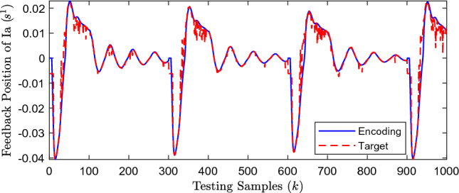
The off-line encoding result of RF

It can be seen from Fig. 7 that the overall effectiveness of the RF-based encoder is very good, the encoding value fits the target value in a straight line at relatively short-term abrupt peak (time 30–40, 60–94, 147–159, 201–211, 287–288, etc); but at relatively long-term abrupt peak (time 7–29, 41–61, etc.) and relatively flat places (time 95–146, 160–200, 212–286, etc.) fits the target values perfectly in a curve, and there is almost no gap between the encoding values and target values. The disadvantage of the RF-based encoder is that the trend of encoding values at the beginning of simulation is somewhat different from the target values, and there is a large gap between the encoding values and target values.

The closed-loop BMI system shown in Fig. 6 is constructed by combining with the designed decoders and the above-mentioned RF-based encoder for comparing the on-line decoding performance of different decoders. In the closed-loop BMI system in this paper, the decoder is used to replace the spinal cord circuit in the original model. It can receive the neural activity generated by the “DVV”, “OPV” and “OFPV” neurons in brain area 4, and decode the neural activity into control instruction to control the movement of the “JPV”. The joint position is the output of the “JPV”. The encoder is used to encode the information of joint position to average firing rate about feedback information. Finally, the encoded feedback information is delivered to the “PPV” neurons. It should be noted that the feedback of the sensory position vector transmitted to “IFV” and “SFV” neurons is not considered.

On-line test of decoders

In order to objectively compare the on-line decoding performance of decoders, the on-line test uses the decoder and encoder models obtained by the off-line training, and the input and output variables of the decoder and encoder models remain unchanged. In addition, the dynamic restoration of the joint position from 0.5 to 0.6 is used to compare the decoding performance of decoders, and the value of joint position $P_i$ is used as the index of decoding performance.

Figure 8 shows the on-line test results of eight decoders. Figure 8a, c, e, g and i show the dynamic restore trajectories of the on-line test values of nine decoders and target values, the “Target” in the figure is the value of joint position output in improved SJIT model, the rest are output values of different decoders in closed-loop BMI system. Figure 8b, d, f, h and j show the absolute error between the on-line test values and target values.

Fig. 8.

The comparison of on-line decoding performance. The figure a, c, e, g and i describe the control effectiveness of different decoders on joint position in the closed-loop brain BMI system based on the improved SJIT model. The target represents the target position of the closed-loop brain BMI system. The figure b, d, f, h and j describe the absolute error between the output from the decoder and target

Figure 8a and b show the on-line test effectiveness of decoders based on EKF and WF. It can be seen that the on-line test effectiveness of EKF-based decoder is significantly worse than that of WF-based decoder. During the entire on-line test, the means of their absolute error are respectively 0.040334 and 0.010076. In addition, the restore trajectory trend of these two decoders is slightly later than the target restore trajectory, and the WF-based decoder can follow the target trajectory well after the time 180. The gap with the target trajectory is small about the WF-based decoder. The restore trajectory of EKF-based decoder has a large gap with the target trajectory in the whole restore process, and it is difficult to stabilize at the joint position of 0.6.

Figure 8c and d show the on-line test effectiveness of decoders based on BP and MNLR. It can be seen that they are both significantly better than that of the decoders based on EKF and WF in terms of overall effectiveness, and the means of their absolute error are respectively 0.009016 and 0.007543. However, they are slightly worse than that of the WF-based decoder in terms of the time required for stabilization and final stability error, and the restore trajectory of MNLR-based decoder is slightly better than that of BP-based decoder. In addition, it can be seen from Fig. 8c that the second-half restore trajectory of the BP-based decoder is more curved and jumpy, while that of MNLR-based decoder is similar to a straight line and is more stable.

Figure 8e and f show the on-line test effectiveness of decoders based on SVR and RF. It can be seen that the overall effectiveness of two decoders is a little better than that of decoders based on BP and MNLR, and the means of their absolute error are respectively 0.007604 and 0.005363. They are obviously better than the above four decoders in terms of the time required for stabilization. As can be seen from Fig. 8e and f, the last two-thirds restore trajectory of SVR-based decoder is almost a straight line and it is stable at a certain value that is slightly larger than the target value 0.6, and the absolute error is larger than that of RF-based decoder. In contrast, the last two-thirds restore trajectory of RF-based is a curve that changes up and down the target trajectory.

Figure 8g and h are the on-line test results of decoders based on KNN and LSTM. It can be seen that both two decoders are better than the above six decoders in the trend of restore trajectory and the gap with target trajectory, and the overall effectiveness of decoder based on LSTM is the best. Moreover, the means of absolute error of decoders based on KNN and LSTM are respectively 0.004296 and 0.003231. From Fig. 8g, it can be seen that the decoders based on KNN and LSTM can well follow the target trajectory, and the gap with the target trajectory is small.

Figure 8i and j is the on-line test results of decoders based on PLS. Compared with other decoders, the on-line decoding performance of PLS based decoders is relatively good. It can be seen that the peak time of the PLS based decoder is slightly ahead of the target value, and the maximum error of the peak value reaches 0.002986. In addition, the decoder based on PLS can better follow the position value of the target. The overall control effect is similar to that of SVR-based decoder. Although the effectiveness of the decoder based on PLS is poor in the off-line test, the on-line decoding effectiveness of the decoder based on PLS is better in the closed-loop BMI system. We speculate that the reason for this phenomenon is that PLS regression can better handle data with high correlation of samples.

In order to compare the on-line test effectiveness of eight decoders more clearly and uniformly, the SOSE is also used to compare the on-line decoding performance of eight decoders, and the formula is as follows:

$$\begin{array}{c}\hfill \mathit{SOSE}=\sum _{k=1}^{300}{(P_i(k)-\overline{P_i}(k))}^2\end{array}$$ 55

where $\overline{P_i}(k)$ is the value of target trajectory; $P_i(k)$ is the value of restore trajectory of each decoder.

The on-line test SOSE value of each decoder is shown in Table 3, and is ranked as: LSTM network, KNN, RF, SVR, MNLR, BP neural network, WF, PLS and EKF. It can be seen from Table 3 that the $\mathit{SOSE}$ value of LSTM-based is the smallest, which is at the level of ${10}^{-3}$. In addition, the $\mathit{SOSE}$ values of the decoders based on KNN, RF, SVR, MNLR, BP neural network and WF are all at the level of ${10}^{-2}$, but the KNN-based decoder is better than the other five decoders. The gap between the $\mathit{SOSE}$ value of above 6 kinds of decoder is not much. The EKF-based and PLS-based decoder is relatively poor among the 9 decoders, and their $\mathit{SOSE}$ values are at the level of ${10}^{-1}$.

Table 3.

The similarity of on-line decoding

Number	1	2	3	4	5	6	7	8	9
Principle	LSTM	KNN	RF	SVR	MNLR	BP	WF	PLS	EKF
$\mathit{SOSE}$	$8.5\times {10}^{-3}$	$1.23\times {10}^{-2}$	$2.03\times {10}^{-2}$	$2.22\times {10}^{-2}$	$3.24\times {10}^{-2}$	$4.13\times {10}^{-2}$	$7.48\times {10}^{-2}$	$2.7\times {10}^{-1}$	$9.7\times {10}^{-1}$

Discussion

According to the comparative analysis of the off-line and on-line test, it can be seen that the overall decoding performance of decoders based on EKF and WF are poor in the close-loop BMI system based on the improved SJIT model. The fitting curve has a large gap with the target value in the change place, but it fits the target value well in the flat place and the fitting curve is relatively stable. From the above analysis, it can be seen that the decoders based on filter have a large inertia and is difficult to adapt to instantaneous changes. But it has better decoding performance and is relatively stable in the static state.

According to the comparative analysis of Figs. 5a and 8c, e, i, it can be seen that the decoding performance of the decoders based on MNLR, SVR and PLS are better than that of the decoders based on filter in the change place, and the fitting curve at the flat place is a straight line. However, they cannot dynamically fit the target value, so its generalization ability is too strong to correspond to small changes. From the Figs. 5a and 8c, e, it can be seen that the decoders based on KNN and RF can follow the target value with a curve in the flat place, but the trend of test values of RF-based decoder is not consist with the target value in Fig. 8e. Therefore, the decoders based on the machine learning method may not be able to dynamically respond to small changes in the static state.

From the Figs. 5c, g and 8c, g, it can be seen that the decoding performance of the decoders based on BP and LSTM is better than others. However, the decoders based on BP and LSTM are inferior to decoders based on machine learning methods in the time required for stabilization and amplitude of jump in Fig. 8c, and the decoding performance of the LSTM-based decoder is close to perfect in Fig. 8g. Therefore, the decoder based on LSTM can better handle on-line decoding than others.

Conclusion

In this paper, we design 9 decoder structures based on the improved SJIT model, and build a closed-loop BMI system based on the improved SJIT model by combining the encoder based on the random forest and the decoder designed. By comparing the off-line and on-line decoding performance of decoders based on MNLR, KNN, SVR, PLS, RF, BP neural network, LSTM neural network, WF and KF, it can be seen that the off-line decoding performance of RF-based decoder is the best, and the on-line decoding performance of LSTM-based decoder is the best. In addition, filter-based decoders are good at handling static decoding processes, decoders based machine learning method are more stable, and ANN-based decoders can better handle dynamic decoding processes. Moreover, the performance of filter-based decoders is poor in general, and that of decoders based on KNN and RF is better among machine learning principles, and the decoding performance of ANN-based decoders varies greatly.

Although our proposed method can effectively compare the decoding capabilities of different decoders for EEG signals, there are some improving future directions.

1. The closed-loop BMI system is difficult to meet the special requirements of complex applications because the control relationship between the decoder and external devices is different from that between the brain and limbs. Therefore, an auxiliary controller is generally introduced in the artificial feedback path to compensate for the difference, so that the BMI system can achieve more accurate control. In the future, auxiliary controllers with different control strategies can be introduced to further optimize the decoding accuracy of the decoder for task instructions in the closed-loop BMI system.

2. Multi-scale neural activity and EEGs are increasingly used as decoded data. For this kind of high-dimensional, high coupling and high complexity signal input, the decoding ability of traditional decoder is limited. Therefore, it is necessary to study the adaptive nonlinear decoder model from the algorithm structure of the decoder in the future.

Funding

This work is supported by the National Natural Science Foundation of China (51905416, 51804249), Xi’an Science and Technology Program (2022JH-RGZN-0041), Qin Chuangyuan “Scientists + Engineers” Team Construction in Shaanxi Province (2022KXJ-38), Natural Science Basic Research Program of Shaanxi (2021JQ-574), Scientific Research Plan Projects of Shaanxi Education Department (20JK0758).

Data availability

The data that support the findings of this study are available on request from the corresponding author Hongguang Pan (hongguangpan@163.com). The data are not publicly available due to the containing information that could compromise research participant privacy.

References

- Ahmadi A, Khorasani A, Shalchyan V, Daliri MR (2020) State-based decoding of force signals from multi-channel local field potentials. IEEE Access 8:159089–159099 10.1109/ACCESS.2020.3019267 [DOI] [Google Scholar]
- Bablani A, Edla DR, Dodia S (2018) Classification of EEG data using k-nearest neighbor approach for concealed information test. Proc Comput Sci 143:242–249 10.1016/j.procs.2018.10.392 [DOI] [Google Scholar]
- Balamurugan B, Mullai M, Soundararajan S, Selvakanmani S, Arun D (2020) Brain-computer interface for assessment of mental efforts in e-learning using the non-Markovian queueing model. Comput Appl Eng Educ 29(4):22209–12220917 [Google Scholar]
- Bullock D, Cisek P, Grossberg S (1998) Cortical networks for control of voluntary arm movements under variable force conditions. Cerebral Cortex (New York, NY: 1991) 8(1):48–62 [DOI] [PubMed] [Google Scholar]
- Chao ZC, Nagasaka Y, Fujii N (2010) Long-term asynchronous decoding of arm motion using electrocorticographic signals in monkey. Front Neuroeng 3 [DOI] [PMC free article] [PubMed]
- Cheng L, Liu Y, Hou Z-G, Tan M, Du D, Fei M (2019) A rapid spiking neural network approach with an application on hand gesture recognition. IEEE Trans Cogn Dev Syst 13(1):151–161 10.1109/TCDS.2019.2918228 [DOI] [Google Scholar]
- Chu Y, Zhao X, Zou Y, Xu W, Song G, Han J, Zhao Y (2020) Decoding multiclass motor imagery EEG from the same upper limb by combining Riemannian geometry features and partial least squares regression. J Neural Eng 17(4):046029 10.1088/1741-2552/aba7cd [DOI] [PubMed] [Google Scholar]
- Dethier J, Nuyujukian P, Ryu SI, Shenoy KV, Boahen K (2013) Design and validation of a real-time spiking-neural-network decoder for brain–machine interfaces. J Neural Eng 10(3):036008–103600813 10.1088/1741-2560/10/3/036008 [DOI] [PMC free article] [PubMed] [Google Scholar]
- Di GQ, Wu SX (2015) Emotion recognition from sound stimuli based on back-propagation neural networks and electroencephalograms. J Acoust Soc Am 138(2):994–1002 10.1121/1.4927693 [DOI] [PubMed] [Google Scholar]
- Dong EZ, Li CH, Li LT, Du SZ, Belkacem AN et al (2017) Classification of multi-class motor imagery with a novel hierarchical SVM algorithm for brain–computer interfaces. Med Biol Eng Comput 55:1809–1818 10.1007/s11517-017-1611-4 [DOI] [PubMed] [Google Scholar]
- Foodeh R, Ebadollahi S, Daliri MR (2020) Regularized partial least square regression for continuous decoding in brain–computer interfaces. Neuroinformatics 18(3):465–477 10.1007/s12021-020-09455-x [DOI] [PubMed] [Google Scholar]
- Gamal M, Mousa MH, Eldawlatly S, Elbasiouny SM (2021) In-silico development and assessment of a Kalman filter motor decoder for prosthetic hand control. Comput Biol Med 132:104353 10.1016/j.compbiomed.2021.104353 [DOI] [PMC free article] [PubMed] [Google Scholar]
- Huang D, Yang C, Pan Y, Cheng L (2019) Composite learning enhanced neural control for robot manipulator with output error constraints. IEEE Trans Ind Inf 17(1):209–218 10.1109/TII.2019.2957768 [DOI] [Google Scholar]
- Jin H, Zhang Z (2013) Research of movement imagery EEG based on Hilbert–Huang transform and BP neural network. J Biomed Eng 30(2):249–253 [PubMed] [Google Scholar]
- Kim S, Sanchez JC, Rao YN, Erdogmus D et al (2006) A comparison of optimal MIMO linear and nonlinear models for brain–machine interfaces. J Neural Eng 3(2):145–161 10.1088/1741-2560/3/2/009 [DOI] [PubMed] [Google Scholar]
- Kobler RJ, Sburlea AI, Mondini V, Hirata M, Müller-Putz GR (2020) Distance-and speed-informed kinematics decoding improves M/EEG based upper-limb movement decoder accuracy. J Neural Eng 17(5):056027 10.1088/1741-2552/abb3b3 [DOI] [PubMed] [Google Scholar]
- Kumar G, Schieber MH, Thakor NV, Kothare MV (2013) Designing closed-loop brain-machine interfaces using optimal receding horizon control. In: 2013 American control conference, pp 5029–5034
- Lebedev MA, Nicolelis MAL (2006) Brain–machine interface: past, present and future. Trends Neurosci 29(9):536–546 10.1016/j.tins.2006.07.004 [DOI] [PubMed] [Google Scholar]
- Li Z, O’Doherty JE, Hanson TL, Lebedev MA, Henriquez CS et al (2009) Unscented Kalman filter for brain–machine interfaces. PLOS ONE 4(7):6243–1624318 10.1371/journal.pone.0006243 [DOI] [PMC free article] [PubMed] [Google Scholar]
- Li Z, O’Doherty JE, Lebedev MA, Nicolelis MAL (2014) Adaptive decoding for brain–machine interfaces through Bayesian parameter updates. Neural Comput 23(12):3162–3204 10.1162/NECO_a_00207 [DOI] [PMC free article] [PubMed] [Google Scholar]
- Lotte F, Bougrain L, Cichocki A, Clerc M, Congedo M, Rakotomamonjy A, Yger F (2018) A review of classification algorithms for EEG-based brain-computer interfaces: a 10 year update. J Neural Eng 15(3):031005 10.1088/1741-2552/aab2f2 [DOI] [PubMed] [Google Scholar]
- Makin JG, Moses DA, Chang EF (2020) Machine translation of cortical activity to text with an encoder–decoder framework. Nat Neurosci 23(4):575–582 10.1038/s41593-020-0608-8 [DOI] [PMC free article] [PubMed] [Google Scholar]
- Mousa FA, El-Khoribi RA, Shoman ME (2016) A novel brain computer interface based on principle component analysis. Proc Comput Sci 82:49–56 10.1016/j.procs.2016.04.008 [DOI] [Google Scholar]
- Nakagome S, Luu TP, He YT, Ravindran AS, Contreras-Vidal JL (2020) An empirical comparison of neural networks and machine learning algorithms for EEG gait decoding. Sci Rep 10(1):4372–1437217 10.1038/s41598-020-60932-4 [DOI] [PMC free article] [PubMed] [Google Scholar]
- Orset B, Lee K, Chavarriaga R, Millan JDR (2020) User adaptation to closed-loop decoding of motor imagery termination. IEEE Trans Biomed Eng 68:3–10. 10.1109/TBME.2020.3001981 10.1109/TBME.2020.3001981 [DOI] [PubMed] [Google Scholar]
- Pan H-G, Wang M, Wang Z-Y, Wang P (2016) The performance comparison of two kinds of decoders in brain–machine interface. In: 2016 International Symposium on Computer, Consumer and Control (IS3C). IEEE, pp 247–250
- Pan HG, Mi WY, Lei XY, Deng J (2020) A closed-loop brain–machine interface framework design for motor rehabilitation. Biomed Signal Process Control 58:101877–11018779 10.1016/j.bspc.2020.101877 [DOI] [Google Scholar]
- Pan HG, Mi WY, Lei XY, Zhong WM (2020) The closed-loop BMI system design based on the improved SJIT model and the network of Izhikevich neurons. Neurocomputing 401:271–280 10.1016/j.neucom.2020.03.047 [DOI] [Google Scholar]
- Pan H, Mi W, Wen F, Zhong W (2020) An adaptive decoder design based on the receding horizon optimization in BMI system. Cogn Neurodyn 14(3):281–290. 10.1007/s11571-019-09567-4 10.1007/s11571-019-09567-4 [DOI] [PMC free article] [PubMed] [Google Scholar]
- Pan H, Mi W, Song H, Liu F (2021) A universal closed-loop brain-machine interface framework design and its application to a joint prosthesis. Neural Comput Appl 33(11):5471–5481 10.1007/s00521-020-05323-6 [DOI] [Google Scholar]
- Pan H, Mi W, Zhong W, Sun J (2021) A motor rehabilitation BMI system design through improving the SJIT model and introducing an MPC-based auxiliary controller. Cogn Comput 13(4):936–945 10.1007/s12559-021-09878-x [DOI] [Google Scholar]
- Pan H, Song H, Zhang Q, Mi W, Sun J (2022) Auxiliary controller design and performance comparative analysis in closed-loop brain–machine interface system. Biol Cybern 116(1):23–32. 10.1007/s00422-021-00897-3 10.1007/s00422-021-00897-3 [DOI] [PubMed] [Google Scholar]
- Pan H, Song H, Zhang Q, Mi W (2022) Review of closed-loop brain–machine interface systems from a control perspective. IEEE Trans Hum Mach Syst 1–17, 10.1109/THMS.2021.3138677
- Robinson N, Vinod AP, Ang KK, Tee KP (2013) EEG-based classification of fast and slow hand movements using Wavelet-CSP algorithm. IEEE Trans Biomed Eng 60(8):2123–2132 10.1109/TBME.2013.2248153 [DOI] [PubMed] [Google Scholar]
- Romero-Laiseca MA, Delisle-Rodriguez D, Cardoso V, Gurve D et al (2020) A low-cost lower-limb brain–machine interface triggered by pedaling motor imagery for post-stroke patients rehabilitation. IEEE Trans Neural Syst Rehabil Eng 28(4):988–996 10.1109/TNSRE.2020.2974056 [DOI] [PubMed] [Google Scholar]
- Roy A, Manna R, Chakraborty S (2019) Support vector regression based metamodeling for structural reliability analysis. Probab Eng Mech 55:78–89 10.1016/j.probengmech.2018.11.001 [DOI] [Google Scholar]
- Seraj E, Sameni R (2017) Robust electroencephalogram phase estimation with applications in brain–computer interface systems. Physiol Meas 38(3):501–523 10.1088/1361-6579/aa5bba [DOI] [PubMed] [Google Scholar]
- Shanechi MM (2017) Brain–machine interface control algorithms. IEEE Trans Neural Syst Rehabil Eng 25(10):1725–1734 10.1109/TNSRE.2016.2639501 [DOI] [PubMed] [Google Scholar]
- Shi Y, Zheng X, Zhang M, Yan X, Li T, Yu X (2022) A study of subliminal emotion classification based on entropy features. Front Psychol 13:781448 10.3389/fpsyg.2022.781448 [DOI] [PMC free article] [PubMed] [Google Scholar]
- Soures N, Kudithipudi D (2019) Spiking reservoir networks: brain-inspired recurrent algorithms that use random, fixed synaptic strengths. IEEE Signal Process Mag 36(6):78–87 10.1109/MSP.2019.2931479 [DOI] [Google Scholar]
- Sun YN, Lo PW, Lo B (2019) EEG-based user identification system using 1D-convolutional long short-term memory neural networks. Expert Syst Appl 125(7):259–267 10.1016/j.eswa.2019.01.080 [DOI] [Google Scholar]
- Sussillo D, Nuyujukian P, Fan JM, Kao JC, Stavisky SD et al (2012) A recurrent neural network for closed-loop intracortical brain–machine interface decoders. J Neural Eng 9(2):026027–102602710 10.1088/1741-2560/9/2/026027 [DOI] [PMC free article] [PubMed] [Google Scholar]
- Tseng PH, Urpi NA, Lebedev MA, Nicolelis M (2019) Decoding movements from cortical ensemble activity using a long short-term memory recurrent network. Neural Comput 31(6):1–29 10.1162/neco_a_01189 [DOI] [PubMed] [Google Scholar]
- Varsehi H, Firoozabadi MP (2021) An EEG channel selection method for motor imagery based brain–computer interface and neurofeedback using Granger causality. Neural Netw 133:193–206 10.1016/j.neunet.2020.11.002 [DOI] [PubMed] [Google Scholar]
- Wang P, Jiang A, Liu X, Shang J, Zhang L (2018) LSTM-based EEG classification in motor imagery tasks. IEEE Trans Neural Syst Rehabil Eng 26(11):2086–2095 10.1109/TNSRE.2018.2876129 [DOI] [PubMed] [Google Scholar]
- Xiao ZD, Hu S, Zhang QS, Tian X, Chen YW et al (2019) Ensembles of change-point detectors: implications for real-time BMI applications. J Comput Neurosci 46:107–124 10.1007/s10827-018-0694-8 [DOI] [PMC free article] [PubMed] [Google Scholar]
- Yan SY, Zhao HB, Liu C, Wang H (2012) Brain-computer interface design based on Wavelet packet transform and SVM. In: International Conference on Systems and Informatics, pp 1054–1056
- Yan EL, Song JL, Liu CN, Luan JM, Hong WX (2020) Comparison of support vector machine, back propagation neural network and extreme learning machine for syndrome element differentiation. Artif Intell Rev 53(3):2453–2481 10.1007/s10462-019-09738-z [DOI] [Google Scholar]
- Yu X, Liu CC, Dai JF, Li J, Hou F (2016) Epilepsy electroencephalogram signal analysis based on improved K-nearest neighbor network. J Biomed Eng 33(6):1039–1045 [PubMed] [Google Scholar]
- Yu JH, Chen L, Zhang RR, Wang KH (2016) From static to dynamic tag population estimation: an extended Kalman filter perspective. IEEE Trans Commun 64(11):4706–4719 10.1109/TCOMM.2016.2592524 [DOI] [Google Scholar]
- Zhang JH, Wang BZ, Li T, Hong J (2018) Non-invasive decoding of hand movements from electroencephalography based on a hierarchical linear regression model. Rev Sci Instrum 89(8):084303–108430313 10.1063/1.5049191 [DOI] [PubMed] [Google Scholar]
- Zhang C, Qiao K, Wang LY, Tong L, Hu GE et al (2019) A visual encoding model based on deep neural networks and transfer learning for brain activity measured by functional magnetic resonance imaging. J Neurosci Methods 325:108318–110831823 10.1016/j.jneumeth.2019.108318 [DOI] [PubMed] [Google Scholar]
- Zou Y, Cheng L (2021) A transfer learning model for gesture recognition based on the deep features extracted by CNN. IEEE Trans Artif Intell 2(5):447–458 10.1109/TAI.2021.3098253 [DOI] [Google Scholar]
Associated Data
This section collects any data citations, data availability statements, or supplementary materials included in this article.
Data Availability Statement