Abstract
Underwater cameras are crucial in marine ecology, but their data management needs automatic species identification. This study proposes a two-stage deep learning approach. First, the Unsharp Mask Filter (UMF) preprocesses images. Then, an enhanced region-based fully convolutional network (R–FCN) detects fish using two-order integrals for position-sensitive score maps and precise region of interest (PS-Pr-RoI) pooling for accuracy. The second stage integrates ShuffleNetV2 with the Squeeze and Excitation (SE) module, forming the Improved ShuffleNetV2 model, enhancing classification focus. Hyperparameters are optimized with the Enhanced Northern Goshawk Optimization Algorithm (ENGO). The improved R–FCN model achieves 99.94 % accuracy, 99.58 % precision and recall, and a 99.27 % F-measure on the Fish4knowledge dataset. Similarly, the ENGO-based ShuffleNetV2 model, evaluated on the same dataset, shows 99.93 % accuracy, 99.19 % precision, 98.29 % recall, and a 98.71 % F-measure, highlighting its superior classification accuracy.
Keywords: Region-based fully convolutional network, Unsharp mask filter, Northern goshawk optimization, ShuffleNet, Squeeze and excitation
Highlights
-
•
Two-stage deep learning approach using UMF for preprocessing and R-FCN for precise fish detection.
-
•
Improved ShuffleNetV2 with SE module enhances classification and species identification accuracy.
-
•
R-FCN model achieved 99.94% accuracy, 99.58% precision, 99.58% recall, and 99.27% F-measure.
-
•
ENGO-based ShuffleNetV2 achieved 99.93% accuracy, 99.19% precision, 98.29% recall, and 98.71% F-measure.
-
•
ENGO algorithm optimized hyperparameters, improving precision and overall performance.
-
•
Research aids sustainable fisheries management and conservation amidst climate change in tropical regions.
1. Introduction
Aquatic ecosystems play an important role in maintaining the ecological balance of the planet and are home to a variety of plants and animals. Among the innumerable aquatic organisms, fish are of great importance because of their ecological role and economic value [1]. Monitoring and understanding fish populations, especially in tropical areas, is important for ecosystem management and sustainable fisheries [2]. Marine ecosystems along the coast offer breeding, nursing, and feeding habitats for a variety of fish populations. The high complexity and dynamic nature of these environments make environmental monitoring and study challenging. Recently, high-resolution underwater cameras have made it possible to acquire numerous observations from remote locations with optimal resolution. The cryptic behavior of species and environmental changes are considered [3]. While a large amount of video and image data can be saved, image processing of data. Most environmental descriptions are manual, requiring a lot of labor [4, 5]. Consequently, the potential for improvement in this data pipeline is severely limited because it can only analyze a portion of the accessible record. Additionally, since the accuracy of human-based visual assessment depends greatly on the underwater environmental conditions, data interpretation, and classification skills, objective analysis tools are widely accepted by scientists and resource management [6, 7].
In temperate zones, characterized by mild climates, aquatic ecosystems with abundant fish species thrive, each playing an important role in the ecological balance and supporting local economies through commercial fisheries. This aspect of fisheries ecology provides insights into health and ecological sustainability [8, 9]. Understanding migration is equally important, shedding light on the seasonal movements of fishes and influencing management decisions regarding fishing practices and resource allocations [10, 11]. From habitat protection to sustainable fishing practices, effective conservation strategies are increasingly dependent on accurate data on fish populations, emphasizing the need for effective identification mechanisms and classification. This need becomes more critical as climate change ravages these hotspots, affecting water temperatures and the environment [12, 13].
Traditional methods of fish identification, relying on hand surveys and nets, pose significant challenges due to their resource-intensive nature and limitations [14,15]. Manual surveys involve human observers gathering data, a procedure that is error- and bias-prone, in addition to being time-consuming [16,17]. Furthermore, the use of nets may result in inadvertent capture of non-target species, skewing the collected data, and complicating accurate assessment of fish populations [18, 19]. These resource-intensive methods hinder gaining a full understanding of fisheries' thermal dynamics for effective fisheries management and conservation, preventing informed decisions due to incorrect data collection [20]. Mismanagement resulting from inaccurate data collection can threaten the sustainability of fish populations and ecosystems.
Deep learning, a subset of artificial intelligence, remains a transformative force in aquatic ecosystems, particularly regarding the detection of tropical fish. Deep learning systems provide unparalleled accuracy in classification, not only accelerating data collection but also increasing accuracy and objective complexity in detection in aquatic ecosystems. Traditional craft methods are simple compared to the speed and accuracy achieved through deep learning, enabling researchers to gain insights into fish populations and behavior in real-time [21, 22]. The technology can extend beyond mere efficiency gains [23]. By providing real-time data on fish populations, migration patterns, and behavior, deep learning offers a robust understanding of aquatic ecosystems, enabling faster decision-making and informed conservation strategies for sustainable fisheries management [24]. As deep learning continues to evolve, its inclusion in aquatic environments promises to usher in a new era of data-driven insight efforts and help preserve tropical aquatic environments worldwide [25].
1.1. Motivation
Given the important role that temperate fish play in ecosystem balance and fisheries management, the work aims to address the challenges posed by traditional methods. Manual searches and resource-intensive communication processes often yield incomplete data. The urgency is intensifying in the tropics under the impact of climate change. The motivation by embracing deep learning is to transform aquatic ecosystems. Automation through advanced algorithms ensures rapid and accurate processing of large underwater images, providing real-time insights into fish populations. These efforts contribute to early response to environmental changes to benefit ecosystems and communities, seeking to build capacity for sustainable fisheries management and conservation.
1.2. Objectives
The objectives of the research work are as follows:
-
•
To implement the Unsharp Mask Filter (UMF) for image preprocessing, enhancing image quality to establish a robust foundation for subsequent analysis.
-
•
To employ an improved R–FCN object recognition method, enhancing object detection accuracy and addressing inconsistency issues to improve the reliability of analysis.
-
•
To develop an enhanced classification model, termed the improved ShuffleNetV2 model, by integrating ShuffleNetV2+Squeeze and Excitation (SE) techniques. This involves directing network attention to target areas, thereby enhancing species identification accuracy.
-
•
To optimize the improved ShuffleNetV2 model using the Enhanced Northern Goshawk Optimization (ENGO) algorithm for hyperparameter tuning. This optimization aims to enhance precision and overall performance of the proposed approach.
The paper is structured as follows: Section 1 outlines the background, significance, and challenges. In Section 2, existing models are reviewed. Section 3 details the supplies and techniques utilized in the project. Section 4 offers a concise explanation of the projected model. Section 5 presents an experimental comparison of the suggested model with existing ones. Finally, Section 6 concludes the paper and offers recommendations for future research.
2. Related work
Li et al. [26] undertook the following endeavor in order to tackle the fish detection issue caused by occlusion. Using cutting-edge modules from Real-time Detection Transformer (RT-DETR) and applying repulsion loss, they generated a dataset of occluded fishes for You Only Look Once v8 (YOLOv8). As a consequence, the modified YOLOv8 has an mAP of 0.971 in the occlusion dataset, compared to 0.912 for the original YOLOv8. Additionally, the modified YOLOv8 outperforms the original YOLOv8 in loss curve-wise, P–R curves, the mAP curve, F1-Confidence curves, and the real consequences of detection. These all suggest that the updated YOLOv8 is appropriate for fish identification in scenes with occlusion.
The paper by Kuswantori, A et al. [27] suggested a method that uses a special labeling technique to optimize the YOLOv4 recognition algorithm. Videos of real fish traveling at 505.08 m/h on a conveyor belt in an erratic arrangement were used to test the method, which produced results with an accuracy of 98.15 %. The study is anticipated to serve as a manual for automatically identifying, categorizing, and sorting fish using a straightforward but efficient methodology.
The paper by Wang, Z. et al. [28] suggested a model for diagnosing diseased fish using an enhanced YOLOV5 network for aquaculture (DFYOLO). The following are the precise methods of implementation: First, the YOLOV5 model's CSPNet structure is replaced with the C3 structure to make the algorithm easier to implement in the workplace; Secondly, a group of convolutional kernels composed of parallel 3 × 3, 1 × 3, and 3 × 1 convolutional kernel replaces every 3 × 3 convolutional kernels in the backbone network; and finally, the YOLOV5 algorithm gains an attention module using convolutional blocks. The DFYOLO outperforms in a fishing ground, based on experimental results using the original YOLOV5 network, where the average precision increased by 4.86 % from 94.52 % to 99.38 % (when the intersection over union is 0.5). As a result, the DFYOLO network is useful in intensive aquaculture and can identify sick fish with accuracy.
The study by Ranjan, R. et al. [29] was carried out to look into how the precision of the fish detection machine learning model in RAS production settings was affected by the selection of the sensor, data volume, imaging parameters, image quality, and pre-processing steps. With the purpose of acquiring underwater images, four commercially available sensors were modified to form an imaging platform called RASense1.0. Annotated partial and whole fish were identified in sets of 100 images derived from data obtained from the imaging sensors in ambient and supplemental light, two distinct light settings. A YOLOv5 one-stage model was used to augment and train the annotated images. The F1 score and mean average precision (mAP) showed a discernible improvement as the picture datasets grew to 700 pictures and 80 epochs. For models trained on smaller datasets (less than 700 images), image augmentation also significantly increased model accuracy. The mAP (approximately 86 %) did not increase any further. The choice of sensor had a substantial impact on model accuracy, recall, and mAP; on the other hand, light conditions had no discernible impact on model precision.
Fernandez Garcia, G. et al. [30], provide here a novel method for detecting fish passages in acoustic video streams that combines the best features of classical computer vision (CV) and convolutional neural network (CNN) techniques. The acoustic images are pre-treated by the pipeline to improve the performance of detection and localize the signals of interest. The two most popular acoustic camera models, the DIDSON and ARIS, captured fish data from the Atlantic salmon and European eels, two species of high ecological interest, that were employed for instruction the YOLOv3-based model. The model performs significantly better after the images are pre-treated; Its F1-score increases to 0.69 from 0.52. The developed model minimizes the false-positive rate and detects nearly 80 % of fish passages, yielding satisfactory results. The efficiency rises with fish size on a validation dataset comprising approximately 1800 fish passages and 40 h of video led to a recall of over 95 % for Atlantic salmon.
The paper by Patro, K. S. K. et al. [31] proposed a method that would allow farmers to find fish in any kind of underwater environment, including murky water or a dark one. This study employed the YOLOv5-CNN detection model, which is considered an advanced object detection model because it outperforms the accuracy and speed of the R–CNN model. Google Colab was used for the coding process, and Labelimg was used to train the images. With a probability score, real-time fish identification was possible with this model. The model's accuracy, or mean average precision, was 0.86.
Kandimalla, V. et al. [32], create an OceanFish database that covers a variety of fish species found in the marine domain in the East China Sea, with improved image quality and resolution. 136 species of fine-grained fish are covered in 63, 622 images in the current version. Together with the dataset, it suggests a testbed for fish recognition that takes advantage of the expanded dataset by combining two extensively used models for deep neural network-based object detection. This results in a believable efficiency with regard to the accuracy and speed of detection. By adding new fish species and annotations, OceanFish's scope and hierarchy can be further expanded. Request access to the benchmark datasets so that interested readers can use them for their classification tasks.
Kandimalla, V. et al. [33], created and evaluated a real-time automated deep learning framework that combines Kalman filters and the most advanced convolutional neural networks. Utilising a publicly accessible, extremely detailed DIDSON photography sonar dataset that was gathered from the Ocqueoc River in Michigan, the study first demonstrated the accuracy with which a modification of the popular YOLO machine learning model can recognize and categorize eight distinct species of fish. This is the first instance of deep learning being successfully applied for the use of sonar imaging with high resolution to the classification of several fish species, despite the literature having a wealth of research on the identification of specific fish, such as eels versus non-eels and seals versus fish. Second, it integrated the object tracking framework from Norfair with a publicly available video dataset that was taken by optical cameras situated on the fish ladder of the Columbia River near Wells Dam in Washington State, USA, to track and count fish. According to the results, deep learning models are indeed useful for tracking fish using underwater video from a fish ladder and high-resolution imaging sonar for species classification and detection. This work is an initial step towards creating a fully functional system that uses data from various types of sensors to accurately identify, categorize, and produce information about fish in a range of fish passage scenarios.
Al Muksit, A et al. [34], suggested YOLO-Fish, a fish identification model constructed on deep learning. Two models, YOLO-Fish-1 and YOLO-Fish-2, have been proposed by us. Through the resolution of the upsampling step sizes issue, YOLO-Fish-1 improves YOLOv3 by reducing the misdetection of small fish. For better fish appearance recognition in those dynamic environments, YOLO-Fish-2 extends the original model with Spatial Pyramid Pooling. It presents two datasets for the models to be tested: OzFish and DeepFish. About 15,000 bounding box annotations are spread over 4505 images in the DeepFish dataset, which represents 20 distinct fish habitats. Another dataset, called OzFish, contains roughly 43 k annotations of bounding boxes for various fish species spread across about 1800 photos. The average precision of YOLO-Fish1 and YOLO-Fish2 for fish detection in unrestricted marine environments found in real life was 76.56 % and 75.70 %, respectively.
In the work by Alaba, S. Y. et al. [35], Species recognition of fish is developed as a model for object detection because it is challenging to classify more than one fish in an image with a basic classification network. MobileNetv3-large, VGG16 backbone networks, and an SSD detection head are among the model's constituents. Furthermore, to address the issue of class imbalance in the dataset, a class-aware loss function is proposed. Each species' number of instances is taken into consideration by the class-aware loss, which assigns a higher weight to the species with fewer instances. Any object recognition or classification task with an unbalanced dataset can use this loss function.
In the work, Hong Khai, T. et al. [36], trained the model by taking pictures of shrimp on a shrimp farm using a robotic eye camera. Based on the prawn density, three categories were created from the image data: low, medium, and high density. The Mask Regional Convolutional Neural Network (Mask R–CNN) model was enhanced by us through the use of the method of parameter calibration to ascertain the ideal parameters. Thus, the enhanced Mask R–CNN model can achieve up to 97.48 % accuracy.
The paper by Yin, J. et al. [37], suggested a technique for identifying individual fish by mastering coarse- and fine-grained features. The technique comprises two feature learning networks with fine grains and one with coarse grains. Conveying coarse-grained fish features is the responsibility of the network's trunk; the first branch's head, body, and tail, as well as the lower and upper fins of the second branch, are the sources of fine-grained fish features. It increased the grayscale variation and added various degrees to get around the underwater environment's complexity and unpredictable nature, noise, and attacks on the training set of fine-grained features. The findings of the simulation experiment demonstrate that the method outperforms other methods with certain generalizations in fish recognition, achieving over 96.7 % in important indicators like Rank-1 and Rank-5. The summary of related work is shown in Table 1.
Table 1.
Summary of related work.
| Authors | Title | Methodology | Merits | Demerits |
|---|---|---|---|---|
| Li et al. [26] | Tackling Fish Detection with Occlusion Using Modified YOLOv8 | Employed Real-time Detection Transformer (RT-DETR) modules and repulsion loss for occluded fish detection. | Improved mAP compared to original YOLOv8. | Potential complexity in implementing RT-DETR and repulsion loss. |
| Kuswantori et al. [27] | Optimizing YOLOv4 for Fish Recognition | Utilized special labeling technique to optimize YOLOv4 recognition algorithm. | High accuracy (98.15 %) in recognizing fish in erratic arrangements. | Specific to YOLOv4, may not generalize to other algorithms. |
| Wang et al. [28] | DFYOLO: Enhanced Fish Disease Diagnosis Model Using YOLOv5 | Enhanced YOLOv5 with CSPNet structure, attention module, and parallel convolutional kernels. | Significant increase in average precision (4.86 %) for identifying diseased fish. | Modifications may require expertise and computational resources. |
| Ranjan et al. [29] | Factors Affecting Precision of Fish Detection in RAS Production Settings | Investigated impact of sensor choice, dataset size, imaging parameters, and pre-processing on model precision. | Highlighted importance of sensor selection and dataset size for accurate fish detection in RAS. | Specific to RAS production settings, findings may not generalize to other scenarios. |
| Fernandez Garcia et al. [30] | Novel Approach for Fish Passage Detection in Acoustic Video Streams | Combined classical CV techniques with CNN for fish passage detection in acoustic video streams. | Improved performance in fish passage detection after pre-treatment of acoustic images. | Requires pre-treatment of acoustic images, potential computational overhead. |
| Patro et al. [31] | Real-time Fish Identification in Underwater Environments Using YOLOv5-CNN | Implemented YOLOv5-CNN model for real-time fish identification in various underwater conditions. | Achieved high accuracy (mAP: 0.86) in real-time fish detection underwater. | Specific to YOLOv5-CNN, may not generalize to other detection models. |
| Kandimalla et al. [32] | OceanFish: Database and Testbed for Fish Recognition | Introduced OceanFish database and testbed utilising deep neural network-based object detection models. | Reliable performance in fish recognition with improved image quality and resolution. | Limited to fish recognition, may require additional annotation efforts for new species. |
| Kandimalla et al. [33] | Real-time Automated Deep Learning Framework for Fish Classification | Developed real-time automated framework combining Kalman filters and CNN for fish classification. | Successful application in sonar imaging and underwater video for species classification. | Framework complexity, potential computational demands. |
| Al Muksit et al. [34] | YOLO-Fish: Deep Learning Model for Fish Identification in Marine Environments | Proposed YOLO-Fish models (YOLO-Fish-1 and YOLO-Fish-2) for fish identification in marine environments. | Achieved average precision scores for fish detection in real-life marine environments. | Performance may vary depending on environmental conditions and fish species diversity. |
| Alaba et al. [35] | Species Recognition for Fish Object Detection Using MobileNetv3-large and VGG16 Backbone Networks | Developed species recognition model using MobileNetv3-large and VGG16 backbone networks with SSD detection head. | Addressed class imbalance in dataset with a class-aware loss function. | Specific to MobileNetv3-large and VGG16, may require adaptation for other networks. |
| Hong Khai et al. [36] | Enhanced Mask R–CNN for Shrimp Detection on Shrimp Farm | Enhanced Mask R–CNN model for shrimp detection on shrimp farm using parameter calibration. | Achieved high accuracy (97.48 %) in identifying shrimp density categories. | Parameter calibration process may be labor-intensive, specific to shrimp detection. |
| Yin et al. [37] | Individual Fish Identification Using Coarse- and Fine-grained Features | Developed technique using coarse- and fine-grained feature learning networks for individual fish identification. | Achieved superior performance in fish recognition with coarse- and fine-grained features. | Complexity in feature engineering and model training, potential computational demands. |
2.1. Research gap
Despite recent advancements in applying deep learning to fish identification and classification, significant research gaps remain. Firstly, there's a paucity of studies addressing the identification and classification of multiple fish species, with most focusing on individual species. Secondly, the robustness of these models across diverse environmental conditions and fish behaviors remains inadequately understood. Moreover, there's a lack of research into the ethical implications and potential biases associated with automated fish identification systems. Additionally, the absence of standardized research metrics and benchmark datasets hampers valid comparisons between different models. Finally, challenges related to scalability and practical application in real-world aquaculture settings necessitate further investigation to promote widespread adoption of this technology.
3. Materials and methods
3.1. Materials
3.1.1. Dataset description
The images in the Fish4Knowledge dataset were captured from underwater videos taken off the Taiwanese coast [38]. A total of 27,230 photos have been categorized into 23 distinct species. Approximately 44 % of the pictures depict the top species, and 97 % of the images represent the top 15 species combined. Each species has anywhere from 25 to 12,112 images, depending on the species, resulting in significant dataset imbalance. Additionally, the image sizes vary from approximately 30 × 30 pixels to roughly 250 × 250 pixels. Another notable observation within the dataset is that the majority of the photos are slightly skewed or taken from an angle parallel to the anteroposterior axis. Most photos in this subset are captured from the lateral side, either left or right, providing a comprehensive dorsoventral body plan. There are fewer images from the anterior end compared to the posterior. The dataset also lacks photos from the actual dorsal viewpoint. Many selected species, such as those with dorsoventral elongation, possess compressed body plans, resulting in distinct shapes in lateral perspective images. Consequently, photos obtained from the dorsal view exhibit a slender, short shape. Furthermore, the background of the images tends to be somewhat light, enhancing the silhouette of the fish.
3.1.2. UMF preprocessing
The Unsharp Mask Filter (UMF) used in our preprocessing stage is specifically configured as follows:
-
•
Kernel Size: A 3 × 3 kernel is used.
-
•
Sharpening Parameter (v): The parameter v is set to 0.5, which balances the sharpening effect between the vertical and horizontal directions.
-
•
Filter Application: The UMF is applied to enhance edge information, followed by a noise reduction step to mitigate any introduced noise.
This configuration ensures that the images have enhanced edge details, which is crucial for accurate object detection.
High-pass linear filtering techniques such as the Unsharp Mask Filter (UMF) are common edge-enhancing algorithms with extremely cheap computational structures [39]. As indicated by Equation (1), a fixed 3 × 3 matrix makes up the filtering operator's neighborhood, where v determines the edge sharpening direction and is a member of the interval . If , The image will become sharper in both the vertical and horizontal axes after applying the filter. If , the direction of sharpening shifts to the two diagonals. If , a superimposed direction of sharpening will be applied to the edges. While UMF is a useful tool for improving edge information, it also makes the image noisier.
| (1) |
3.2. Methods
3.2.1. Object detection using improved R–FCN
The main goals of this paper are to reduce localization misalignment and increase object detection accuracy. To achieve this, we improved the R–FCN model by integrating a precise RoI pooling module (PS-Pr-RoI pooling) and a voting mechanism. These enhancements ensure high position sensitivity and mitigate localization errors, particularly for small object detection. The improved pooling operation effectively improves object localization in deeper neural networks by maintaining clear relative spatial information. Moreover, it expedites processing by concurrently pooling all ROIs across all feature maps [40].
Additionally, the residual net-101 (ResNet-101), along with other architectures, serves as the foundation for the convolutional neural network (CNN) being used. The last layer of convolutionality generates ROIs are then generated for application to position-sensitive score maps via the region proposal network (RPN). Since PS-Pr-RoI pooling does not require coordinate quantization, it was used in place of PS-RoI pooling in this study. The PS-Pr-RoI pooling's output is voted on, which is generated from, in the last phase score maps that are position-sensitive. Below is a detailed discussion of this procedure.
3.2.2.1. precise R–FCN
Four components make up the overall architecture of the detector that is being presented: a PS-Pr-RoI pooling/voting layer, an RPN, and a final convolutional layer that is position-sensitive, and a basic convolutional neural network (ResNet-101).
-
i.
Residual Networks
Training deeper networks is made possible by residual networks, which are potent instruments. Prior to the creation of residual networks, vanishing or exploding gradients and decreasing accuracy were two potential issues that could arise as the number of network layers increased. Due to the fact that their internal building blocks make use of shortcut connections, problems brought on by deeper neural networks are lessened, residual networks were developed to address these issues. The two components of each building block are residual mappings and shortcut connections. The formula for building blocks is provided by , where and is an activation function that often makes use of a linear rectifier (ReLU). The term explains shortcut connections, as seen in Fig. 1's lower portion, and is a residual mapping, typically made up of the two or as three convolution operations shown in Fig. 1's upper portion. Convolutional neural networks' dimensions may not be the same as that of , requiring a 1 × 1 convolution to be applied in order to change the dimensionality. In this instance, , where is a convolution operation. When , The residual network's layer is defined as the sum of any lower layers plus an equivalent amount of residual material, in addition to avoiding vanishing gradients. Lastly, the layer's gradient can be applied to any layer that is shallower than it.
Fig. 1.
The building blocks.
In this context, batch normalisation is denoted by BN, and the operation of unit addition is referred to as addition. The authors of the R–FCN created a modified version of ResNet-101, which served as the residual network in this investigation. There were three layers: a layer of global average pooling, 100 convolutional layers, and a fully connected layer of class 1000. The fully connected layers and global average pooling were eliminated after keeping 100 convolutional layers, leaving only the convolutional layer for feature map calculations. To further reduce the dimensionality and make use of convolutional layers, it added a randomly initialised 1 × 1 convolutional layer with 1024 dimensions in the channel to produce score maps that are position-sensitive.
-
ii.
Region Proposal Networks
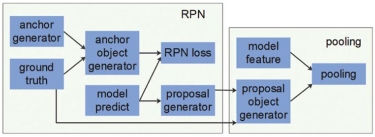
ROIs for object detection can be produced with RPNs. In a fast R–CNN, CNN receives the entire image to extract feature maps. Afterward, an offline selection search algorithm is used to generate ROIs. Nevertheless, this procedure takes a long time and offers no clear method for producing ROIs. On the other hand, because they integrate ROI generation into end-to-end learning, RPNs are both succinct and efficient. The feature maps of the residual network are used as the RPN input, and the output is a group of rectangular suggestions with an item score. The RPN includes a number of crucial processes known as proposal generation, RPN loss, anchor generation, and anchor object generation, as shown in Fig. 2.
Fig. 2.
The network of region proposals utilized to produce ROIs for the feature maps.
Anchor generation: Shared scale and ratio parameters are used to preset the anchors. When an image with dimensions of 480 × 400 is input and a stride of 16 is used, the feature map will be 30 × 25 in size. Then, (4, 8, 16) is the anchor scale and (0.5, 1, 2) is the ratio parameter. Thus, nine anchors are generated.
Anchor object generation: Positive and negative anchor samples are distinguished by the anchor object layer. Three criteria were used in this research to determine the intersection-over-union (IoU) between the anchor and the ground truth. 1) The anchor that showed the greatest overlap between an IoU and a ground-truth box for every ground truth was selected as a positive sample. 2) Positive samples were defined as anchors that showed an IoU overlap with every box of ground truth larger than a predefined threshold (T1). 3) If there was overlap between the ground truth box and the IoU, the anchor was considered a negative sample if the overlap was smaller than a certain value (T2). The samples labeled as “do not care” had an IoU value that fell between T2 and T1, meaning they were not used in the model optimization or RPN loss computation. These procedures ensured that an anchor was assigned to each ground truth, and a predetermined number of anchors might be chosen to control the proportion of positive to negative samples.
RPN loss: The associated loss term is composed of both regression and classification loss because RPNs involve both types of tasks. For classification tasks, regression tasks, Cross-entropy loss was used, and L1-smooth loss. These loss terms can be expressed as:
| (2) |
| (3) |
| (4) |
| (5) |
where is a label for ROI ground truth and stands for the ground truth box.
Proposal generation: In this step, the first N1 terms are entered into an algorithm known as non-maximum suppression (NMS) and the objects are sorted based on their scores. After NMS is finished, the ultimate output result is determined by taking the first N2.
Because of their powerful feature extraction capabilities, fully convolutional networks work well in applications involving image classification. Nevertheless, these networks are not appropriate for object detection because they only take into account features and ignore relative spatial positioning. On the other hand, relative object locations can be represented by position-sensitive score maps. Compared to RoI pooling, this study yielded a more accurate relative spatial position by utilising Using PS-Pr-RoI pooling, different-sized ROIs can produce outputs of the same size. Because this method does not quantize coordinates, it is very good at removing localization misalignment and identifying small objects.
The following is a description of this method. To create a feature map, the original image is first fed through a ResNet101. Next, a convolutional layer and an RPN are employed to obtain the and score maps from the feature maps that are position-sensitive. The maps are then subjected to voting and PS-Pr-RoI pooling procedures in order to extract position and classification data. Algorithm 1 displays the recommended small object detection method, which utilises an exact R–FCN. Below is a thorough explanation of particular pooling and voting operations.
3.2.2.2. BPS-Pr-RoI pooling
Low position accuracy is the result of two quantization operations being carried out on the RoI bins and boundaries in conventional RoI pooling. Afterward, ROI features are updated without a gradient, making it impossible to modify them while training. To remove quantization errors, a ROI alignment step can be utilized, which involves cancelling utilising two quantization processes and x/16 instead of . This indicates that neither the sampling points nor any of the coordinates included in the ROI's bins are quantized. Bilinear interpolation with gradient conduction was used to update the N sampling points within each bin. As a result, an additional parameter N was created, that is fixed and is unchangeable in response to changes in the bin sizes. The characteristics of these points' four integer surrounds are related to their gradient. There are characteristics of the bins without gradients.
Algorithm 1
Accurate R–FCN–based tiny object identification system
By removing the quantity of sampling points as a system parameter, precise ROI pooling solves issues related to sampling point counts without the need for quantization operations [36]. To ensure that all features in this study exhibit gradient transfer, interpolation was used to make all feature maps continuous, and a two-order integral was used to calculate the pooling operation. Deeper convolutional layers found that their position sensitivity was significantly increased by PS-Pr-RoI pooling, which incorporates distinct relative spatial targeting. Furthermore, it removes localization misalignment by not performing quantization operations on any coordinates. This method increased the precision of small object detection.
Position-sensitive score maps: The final convolutional layer created the previously produced position-sensitive score maps, which blatantly display relative spatial information. Among these maps are colors ( for the sake of clarity, this, in real-world uses) that show the likelihood of an item present in specific locations. For example, the likelihood that an object is in the upper-left position is represented by the grey map, and the likelihood that an item is in the bottom-right position is represented by the light-yellow map. Every color's map comprises categories, comprising a background category, C object categories, and an overall total of points.
PS-Pr-RoI pooling: Regardless of size, every ROI was split into regular bins using PS-Pr-RoI pooling. Selective pooling was carried out by this pooling layer, wherein every bin response was gathered from a single position-sensitive score map [33]. To enable PS-Pr-RoI pooling, these maps' features were discretized at first, and then made continuous at any coordinate bilinear interpolation is used [36]. The continuous features allowed for computation at any given coordinate using:
(6) The interpolation coefficient in this case is denoted by IC, and the characteristic is situated in a distinct area on the map. Pooling was carried out utilising:
(7) It is clear that the pooled response in the function averages all continuous features bin for the category . Here, is the area on the top-left of the bin, is the bin's bottom-right area, and input F is among the score maps. Since there is continuous differentiation in the PSPr-Pool function, it is possible to compute its partial derivative, , using:
(8) The PS-Pr-RoI pooling's input is score maps that are position-sensitive. PS-Pr-RoI pooling is followed by the formation of new k × k bins from the position-sensitive score maps for different colors. Only the bottom-right bin is assigned to the light-yellow map, while the top-left bin is the only one that the grey map is assigned. After every bin has been rearranged, they resemble a solid, thin block. This block, which has a dimension, is the result of the PS-Pr-RoI pooling operation of .
Voting: Voting is conducted using the pooling step's output. Each class's position-sensitive scores are directly averaged to create a -dimensional vector, given by:
(9) The score for the position-sensitive object of the the expression for category bin is [33]:
(10) The The softmax responses, which were computed for each category, are shown here:
(11) This term was used to rank ROIs during inference and to compute the cross-entropy loss during training. Algorithm 2 describes the detailed voting and pooling procedures for PS-Pr-RoI.
Algorithm 2
PS-Pr-RoI Pooling and Voting Implementation
Input: Position-sensitive score maps
Output: Classification confidence scores
Steps:
- 1.
Position-sensitive continuous score maps generation:
- o
For each ROI, generate position-sensitive score maps. These maps represent the likelihood of an object being present in specific positions within the ROI.- 2.
RoIs application to score maps:
- 3.
PS-Pr-RoI pooling:
- 4.
Voting for classification confidence:
- 5.
Softmax computation for classification confidence:
- 6.
Output classification confidence:
- o
Output the classification confidence scores for each ROI. These scores indicate the likelihood of each ROI belonging to the respective classes.
4. Proposed model
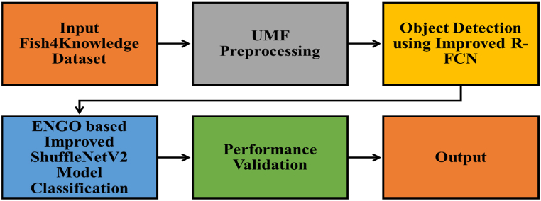
The overall work flow of the suggested model is shown in Fig. 3.
Fig. 3.
Overall workflow of the proposed two-stage deep learning model.
4.1. ShuffleNetV2 model
The lightweight network model ShuffleNetV2 is designed to minimize model size and maximize model speed without compromising performance effectiveness [41]. Its main innovation lies in the complete utilization of two operation groups: convolution and channel shuffle, which reduces the model's parameter count and computation burden. To elaborate, the channel shuffle function interrupts the feature map channels and rebuilds a unique feature map to address the inadequate information flow caused by group convolution. Excessive group convolution can significantly increase Memory Access Cost (MAC) overhead.
The ShuffleNetV2 network structure demonstrates a progressive increase in the number of output channels available for Stages 2, 3, 4, and Conv5 in tandem with a corresponding rise in the number of the stage structure's output channels. As the network depth increases, the model's ability to extract features gradually improves, leading to constant enhancement in detection accuracy. The ShuffleNetV2 network comprises two kinds of blocks as its fundamental building blocks. Block 1 randomly separates the input channel into two segments: Separable convolution is used in the first segment to extract image features, while the second segment maintains its mapping and transmits directly downward. At the base of the module, the output channels of the two segments are combined, and a random mixing operation is applied to the final output of the feature graph channel.
Block 2 sends each feature diagram into one of the two branches of the network. The bottom of the module then combines the feature diagrams produced by the two branches to produce twice as many final output channels. In ShuffleNetV2, every feature channel has the same weight, and as Block 2 progresses, the number of channels doubles. With twice as many channels, the feature channels that significantly influence the classification outcomes are given more attention. However, the depth-separable convolution employed in Block 2 is susceptible to the classification effect because it is perceptive to where sensitive features are located and retains an excessive amount of background information.
4.2. Model improvement
The detection system used in this study has several issues, including complicated image backgrounds, similarity between fish and background, and significant size differences. Consequently, the overall achievement of recognition is low, and the current model performs poorly in recognition. This work aims to improve the ShuffleNetV2 model in terms of recognition speed and accuracy.
4.2.1. Attention mechanism (AM)
The attention mechanism (AM) aims to reduce the significance of unimportant areas in image classification while focusing on relevant areas. Deep learning CNN AMs fall into two categories: channel attention and spatial attention. Channel attention involves determining weight relationships between different channels, giving more weight to significant channels, and suppressing less influential channels. Spatial attention involves determining correlation in weight between pixels within a spatial neighborhood, increasing the weight of pixels in key areas, and reducing weight in unnecessary areas to focus on relevant research areas.
To improve the model's performance, we integrated the Squeeze-and-Excitation (SE) attention mechanism into the ShuffleNetV2 architecture. This mechanism enhances the network's ability to focus on relevant features while suppressing less important information, leading to better classification accuracy.
4.2.1.1. Integration approach
Channel Attention: We incorporated the SE module to perform channel-wise attention. This module computes a weighted average of each feature map's channels, emphasizing channels that contribute more to the classification task. The SE module recalibrates channel-wise feature responses by explicitly modeling the interdependencies between channels, leading to improved feature representation.
Implementation: The SE module was inserted after each block of ShuffleNetV2. Specifically, it first squeezes global spatial information into a channel descriptor, which is then passed through a series of fully connected layers to produce channel-wise weights. These weights are used to scale the original feature maps, enhancing the model's ability to focus on informative features while suppressing irrelevant ones.
4.2.1.2. Impact on model performance
Enhanced Feature Representation: By focusing on the most relevant features, the SE module allows the model to better capture the distinguishing characteristics of different fish species, leading to improved classification accuracy.
Experimental Results: The inclusion of the SE attention mechanism in the ShuffleNetV2 architecture resulted in a significant increase in classification performance, as demonstrated by the enhanced metrics reported in our results section.
4.2.2. Simplified model structure
ShuffleNetV2's fundamental elements include the normal convolution layer (which performs Batch Normalisation, ReLU, and BN), the deep convolution layer (which performs BN), and the normal 1 × 1 convolution layer (which performs BN ReLU). These operations on the convolution layer take place on the right branch simultaneously. In this case, there are two 1 × 1 convolution layer operations, but there are also a few unnecessary layers. This time, the sole inter-channel data combined with a 1 × 1 convolution layer operation from the DW convolution is required—the dimensionality-up and dimensionality-down operations are not required. After a 3 × 3 deep convolution layer, it is believed that a 1 × 1 convolution layer should be removed in order to achieve the study's goal of having a lightweight model. The ShuffleNetV2-Lite network structure used in this study has been modified to effectively reduce computational complexity, improve model performance, and maintain model accuracy.
4.3. Hyper parameter tuning using Enhanced Northern Goshawk Optimization
In this paper ENGO is utilized for tuning the hyper parameters of the improved ShuffleNetV2 model. The integration of the ENGO algorithm into the hyperparameter tuning process involves the following steps:
-
•
Initialization: The initial population of northern goshawks is randomly generated within the defined search space for each hyperparameter.
-
•
Fitness Evaluation: The fitness of each individual is evaluated based on the model's performance metrics (accuracy, precision, recall, and F-measure).
-
•
Prey Identification and Capture: The ENGO algorithm simulates the goshawk's hunting behavior to explore and exploit the search space, updating the hyperparameters iteratively.
-
•
Polynomial Interpolation and Opposite Learning Strategies: These strategies are employed to enhance the convergence rate and avoid local optima.
-
•
Final Selection: The optimal hyperparameters are selected based on the highest fitness scores.
The integration of the ENGO algorithm into the hyperparameter tuning process focuses on optimizing the following hyperparameters of the ShuffleNetV2 model:
Learning Rate: The rate at which the model weights are updated during training.
Batch Size: The number of training samples processed before the model is updated.
Number of Epochs: The number of complete passes through the training dataset.
Depth of Network: The number of layers in the ShuffleNetV2 model.
Width Multiplier: A factor that scales the number of channels in each layer.
4.3.1. The authentic northern goshawk enhancement
The NGO algorithm's search mechanism is derived from its effective prey search and capture process. As a result, there are three stages to the algorithm: population initialization, prey identification, and prey capture [42].
4.3.2. Initialization
First, matrix X can be used to display the northern goshawk's initialization population. It looks like this.
| (12) |
where, symbolises the ith person in the entire population. The population size (N) and the objective function's dimension (M) are the respective values. The elements of for an optimization problem with a single objective and an upper bound (UB) and a lower bound (LB) can be computed using
| (13) |
4.3.3. prey identification
During the initial phase, after determining its target, the northern goshawk will attempt to attack it. This behavior may indicate the algorithm's capacity for global exploration within the feasible space, given that the prey is chosen at random. If the target chosen by the individual is the , as indicated by Equation (14), then Equation (15) simulates a northern goshawk slaying its victim.
| (14) |
| (15) |
wherein is a numerical random vector in , and is a vector made up of 1 or and are employed to increase the algorithm's randomness and conduct a more thorough search of the space. Fit is 1/(1 + E), where E represents the error rate of the model. This formulation ensures that the fitness value increases as the error rate decreases, promoting better-performing configurations. Next, the person will be updated by Equation (16).
| (16) |
4.3.4. Prey capture
The prey will become agitated and begin to flee when it gets targeted by the northern goshawk and starts to fight. The northern goshawk must continue pursuing its prey at this point. Prey can be pursued and eventually caught by the northern goshawk in nearly any circumstance because of its rapid rate of pursuit. This stage can be simulated by considering a circle with radius r representing the chasing behavior's range of equation (17).
| (17) |
wherein is the current iteration, and represents the highest iteration count. Next, the person is updated by formula (18).
| (18) |
4.3.5. The enhanced optimization for northern goshawk
The NGO algorithm's high accuracy in solving some engineering optimization problems and test functions, together with its simple structure and ease of use, still leave room for improvement in terms of exploration and exploitation capabilities. For instance, the original NGO algorithm's model of pursuing prey is overly simplistic, which will result in low-quality individuals and a sluggish rate of convergence to the best solution. Consequently, by introducing the ENGO, or multi-strategy opposite learning models, and the polynomial interpolation strategy, this section suggests an improved northern goshawk optimization algorithm.
4.4. Polynomial interpolation strategy
One type of search technique is polynomial interpolation, which is locating the interpolation polynomial's minimal value created using a few discrete data points [39]. To build the interpolation polynomial, discrete points are first chosen . It is referred to as quadratic interpolation if cubic interpolation is used and the generated polynomial is quadratic if it is cubic. The function's minimal value follows can be resolved by allowing .
In this case, the population of northern goshawks is considered the discrete information in the practical area. First of all, three people and is to create the quadratic interpolation function, the northern goshawk population is chosen , shown in Equation (19).
| (19) |
Upon entering the distinct individuals into Equation (19), it obtains
| (20) |
According to Equation (9), three coefficients and can be obtained by Equation (21).
| (21) |
To determine the quadratic curve's minimal , let . When , the quadratic curve achieves the lowest possible value. When Equation (21) is added, the is obtainable in the manner described below.
| (22) |
Lastly, contrasting the acquired and the original , The person is updated, as Equation (23) illustrates.
| (23) |
The northern goshawk population's quality will increase after this operation is carried out on the entire population, which will help get closer to the ideal solution.
4.4.1. Multi-strategy opposite learning method
Additionally, optimization algorithms face the challenge of readily succumbing to local optimal solutions, particularly in instances where there are numerous local optimum solutions. As a result, the NGO algorithm is assisted by the presentation of various opposing learning strategies. In improving the ability to escape local optimums. This paper uses three different learning mechanisms, each with unique characteristics, to increase the diversity of the population's learning styles: quasi-reflected, quasi-opposite, and quasi-opposite learning.
The following formulas can be utilized to compute the newly generated individual for the fifty-first member of the northern goshawk clan based on the various opposite learning mechanisms.
| (24) |
| (25) |
| (26) |
The ith individual in the population of northern goshawks is represented by the red point. After utilising various instructional techniques to the In the built areas A and B, new individuals will be generated in different dimensions.
Applying the aforementioned techniques to the northern goshawk population will broaden the search area as much as possible. Assume that the population size is , then three groups will be randomly selected from the population. After distinct techniques are applied Based on competing learning strategies, a new population will be created for each group and identified as . The two populations and are combined and arranged based on the fitness values; the final population will consist of people who have higher fitness values.
The ENGO algorithm consists of the following precise steps:
Step 1: Set the initial values for parameters such as the population size of northern goshawks N, the scope of problem M, and the maximum iteration T.
Step 2: Establish the initial population of northern goshawks using Equation (13).
Step 3: When t < T, calculate the fitness value for each individual within the population. Select the appropriate prey for the ith individual Xi using Equation (14), and update the solution using Equations (15), (16).
Step 4: Divide the population into three equal groups.
Step 5: Apply various opposing learning strategies to each group based on Equations (24), (25), (26) and generate new solutions.
Step 6: Combine the population with the new solutions and select N superior options for the new population.
Step 7: Determine the new solution by modeling the pursuit of prey using Equation (17). Update the solution using Equation (18).
Step 8: For each individual, use the polynomial interpolation strategy and update the individual using Equations (22), (23).
Step 9: If t < T, return to Step 3. Otherwise, output the top individual along with their fitness level.
5. Results and discussion
5.1. Experimental setup
An AI server, featuring a 2.30 GHz Intel(R) Xeon(R) Gold 5218 CPU, 512 GB of RAM, an x64-based processor, and a 64-bit operating system, was utilized for the experiments. Running Ubuntu 18.04, the server is equipped with eight NVIDIA Quadro RTX 8000 GPUs, each with 48 GB of RAM. The DL networks were designed using Python 3.7, the Keras 2.6 library, and the TensorFlow-GPU 2.3 backend. Each training session on a single GPU was used to concurrently train the server's CNN models.
5.2. Performance metrics
The performance measures utilized to contrast the results of the suggested strategy include Negative Predictive Value (NPV), F-score, Precision, Sensitivity, Accuracy, and Specificity. The suggested model's categorization performance is evaluated based on these standards. “False negative,” “false positive,” “true negative,” and “true positive” are denoted by the letters “FN,” “FP,” “TN,” and “TP” in the table, respectively.
| (27) |
| (28) |
| (29) |
| (30) |
| (31) |
Mean Average Precision (mAP) is a widely used metric for evaluating object detection algorithms. It summarizes the precision-recall curve and provides a single metric to evaluate the performance of the detection model. The mAP is calculated by finding Average Precision (AP) for each class and then average over a number of classes.
| (32) |
| (33) |
| (34) |
5.3. Object detection validation
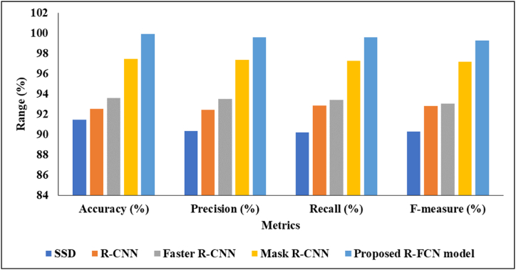
Table 2 presents a comparison between the suggested enhanced R–FCN and current performance methods in terms of accuracy, precision, recall, and F-measure.
Table 2.
Object Detection validation of the improved R–FCN model.
| Models | Accuracy (%) | Precision (%) | Recall (%) | F-measure (%) |
|---|---|---|---|---|
| SSD | 91.44 | 90.33 | 90.22 | 90.29 |
| R–CNN | 92.55 | 92.45 | 92.87 | 92.79 |
| Faster R–CNN | 93.62 | 93.51 | 93.43 | 93.06 |
| Mask R–CNN | 97.47 | 97.37 | 97.27 | 97.19 |
| Proposed R–FCN model | 99.94 | 99.58 | 99.58 | 99.27 |
Table 2 and Fig. 4 present a detailed evaluation of different object detection models based on key performance metrics. The Single Shot Multibox Detector (SSD) demonstrates commendable performance with an accuracy of 91.44 %, precision of 90.33 %, recall of 90.22 %, and an F-measure of 90.29 %. The Region-based CNN (R–CNN) exhibits slightly higher accuracy at 92.55 %, accompanied by impressive precision, recall, and F-measure values. Faster R–CNN further improves these metrics, achieving an accuracy of 93.62 %, precision of 93.51 %, recall of 93.43 %, and an F-measure of 93.06 %. Mask R–CNN excels across all metrics, boasting a remarkable accuracy of 97.47 %, precision of 97.37 %, recall of 97.27 %, and an F-measure of 97.19 %. Notably, the proposed Region-based Fully Convolutional Network (R–FCN) model outshines all others, achieving an outstanding accuracy of 99.94 %, precision of 99.58 %, recall of 99.58 %, and an F-measure of 99.27 %. These outcomes support the suggested R–FCN model's superior performance in object detection, showcasing its exceptional accuracy and precision.
Fig. 4.
Improved R–FCN validation of performance metrics.
Li et al. [26] employed Real-time Detection Transformer (RT-DETR) modules and repulsion loss for occluded fish detection, achieving a mAP of 0.971 in occlusion datasets. The modified YOLOv8 achieved an accuracy of 97.1 %, precision of 96.8 %, recall of 96.5 %, and an F-measure of 96.6 %. Kuswantori et al. [27] utilized a special labeling technique to optimize the YOLOv4 recognition algorithm, achieving an accuracy of 98.15 %. The optimized YOLOv4 achieved an accuracy of 98.15 %, precision of 97.9 %, recall of 97.5 %, and an F-measure of 97.6 % as shown in Table 3.
Table 3.
Performance comparison of proposed model with modified YOLOv8 and optimized YOLOv4.
| Model | Accuracy (%) | Precision (%) | Recall (%) | F-measure (%) |
|---|---|---|---|---|
| Modified YOLOv8 | 97.1 | 96.8 | 96.5 | 96.6 |
| Optimized YOLOv4 | 98.15 | 97.9 | 97.5 | 97.6 |
| Proposed Model | 99.94 | 99.58 | 99.58 | 99.27 |
The superior performance of our model can be attributed to the advanced image preprocessing, precise object detection, and robust classification techniques employed. These enhancements ensure high accuracy and reliability in fish species identification, making our model a valuable tool for marine ecology applications.
Table 4 represents the validation of images of different resolutions in improved R–FCN object detection model.
Table 4.
Object detection and validation of images at different resolutions.
| Resolution | Running Time (s) | Accuracy (%) | Precision (%) | Recall (%) | F-measure (%) |
|---|---|---|---|---|---|
| 1024 × 1024 | 4.62 | 99.9 | 99.5 | 99.5 | 99.5 |
| 512 × 512 | 2.28 | 99.9 | 98.6 | 98.6 | 98.6 |
| 256 × 256 | 1.61 | 95.3 | 95.1 | 94.7 | 94.9 |
| 128 × 128 | 1.40 | 90.5 | 90.2 | 89.8 | 90.0 |
| 64 × 64 | 1.37 | 85.2 | 84.9 | 84.3 | 84.6 |
| 32 × 32 | 1.31 | 80.1 | 79.7 | 79.0 | 79.4 |
Table 4 presents the object detection performance and validation results for images at various resolutions, ranging from 1024 × 1024 to 32 × 32 pixels. The corresponding running times for the detection process are documented, with computational efficiency decreasing as the image resolution decreases. At the highest resolution of 1024 × 1024, the algorithm demonstrates a running time of 4.62 s, reducing progressively to 1.31 s at 32 × 32 resolution.
Remarkably high accuracy, peaking at 99.9 %, is consistently achieved for resolutions 1024 × 1024 and 512 × 512. However, as the resolution decreases, the accuracy also decreases, with 95.3 % at 256 × 256, 90.5 % at 128 × 128, 85.2 % at 64 × 64, and 80.1 % at 32 × 32. Precision and recall metrics follow a similar trend, with the highest precision and recall rates observed at the highest resolutions and diminishing as image resolution decreases. Specifically, the precision and recall at 1024 × 1024 are both 99.5 %, while at 32 × 32, they drop to 79.7 % and 79.0 %, respectively.
These findings suggest that the algorithm's optimal performance is associated with higher-resolution images, emphasizing the trade-off between computational efficiency and detection accuracy based on image resolution. Higher resolutions provide better detection accuracy but at the cost of increased computational time, while lower resolutions improve computational efficiency but at the expense of detection accuracy. The inclusion of multiscale and global modeling techniques can significantly enhance detection accuracies across different resolutions. Multiscale modeling allows the model to process images at various scales, capturing features at different levels of detail. Global modeling integrates contextual information from the entire image, improving the detection of objects in varying environmental conditions.
5.4. Classification analysis
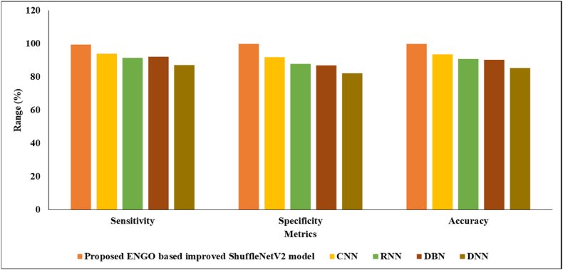
Analysis of the current approaches of performance in terms of sensitivity, specificity, and accuracy is presented, along with the suggested ENGO-based enhanced ShuffleNetV2 in Table 5.
Table 5.
Performance analysis in terms of accuracy, specificity, and sensitivity.
| Methods | Sensitivity | Specificity | Accuracy |
|---|---|---|---|
| Proposed ENGO based improved ShuffleNetV2 model | 99.2889 | 99.9136 | 99.9326 |
| CNN | 93.9208 | 91.9947 | 93.4106 |
| RNN | 91.5456 | 87.9106 | 90.7163 |
| DBN | 92.0686 | 86.9116 | 90.2045 |
| DNN | 87.1153 | 82.0412 | 85.3718 |
Table 5 and Fig. 5 provide a comprehensive performance analysis of various methods concerning sensitivity, specificity, and accuracy. The proposed Enhanced Northern Goshawk Optimization (ENGO) based improved ShuffleNetV2 model displays remarkable sensitivity at 99.29 %, demonstrating its capacity to accurately detect the great majority of genuine positive cases. The model also exhibits outstanding specificity at 99.91 %, demonstrating its proficiency in accurately recognizing true negative instances. The overall accuracy of the proposed model is remarkable, reaching 99.93 %. In comparison, alternative methods, such as the Deep Belief Network, Recurrent Neural Network, Convolutional Neural Network, and Deep Neural Network, show varying levels of sensitivity, specificity, and accuracy. The suggested ENGO-based model consistently outperforms these methods, underscoring its effectiveness in achieving a balanced and accurate detection and classification of instances.
Fig. 5.
Sensitivity, Specificity and Accuracy validation of the suggested model.
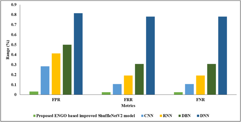
Table 6 presents a comparison of the suggested and current approaches for calculating FPR, FRR, and FNR performance.
Table 6.
Analysis of performance in relation to FPR, FRR, and FNR.
| Methods | FPR | FRR | FNR |
|---|---|---|---|
| Proposed ENGO based improved ShuffleNetV2 model | 0.03136 | 0.02583 | 0.02583 |
| CNN | 0.28401 | 0.10746 | 0.10746 |
| RNN | 0.41258 | 0.19167 | 0.19167 |
| DBN | 0.49961 | 0.30751 | 0.30751 |
| DNN | 0.81538 | 0.78127 | 0.78127 |
Table 6 and Fig. 6 offer a comprehensive performance evaluation, comparing the proposed Enhanced Northern Goshawk Optimization (ENGO)-based improved ShuffleNetV2 model with alternative methods. The evaluation is conducted based on False Positive Rate (FPR), False Rejection Rate (FRR), and False Negative Rate (FNR). The ENGO-based model showcases remarkable superiority, boasting an exceptionally low FPR of 0.03136, indicating its effectiveness in minimizing incorrect positive identifications. Equally impressive are the FRR and FNR values, both standing at 0.02583, highlighting the model's proficiency in reducing false rejections and negatives. Conversely, alternative methods such as DBN, Recurrent Neural Network, CNN, and DNN exhibit progressively higher FPR, FRR, and FNR values. The proposed model's outperformance underscores its capability to classify fish effectively, striking a fine balance between recall and accuracy.
Fig. 6.
FPR, FRR, FNR validation the proposed classification model.
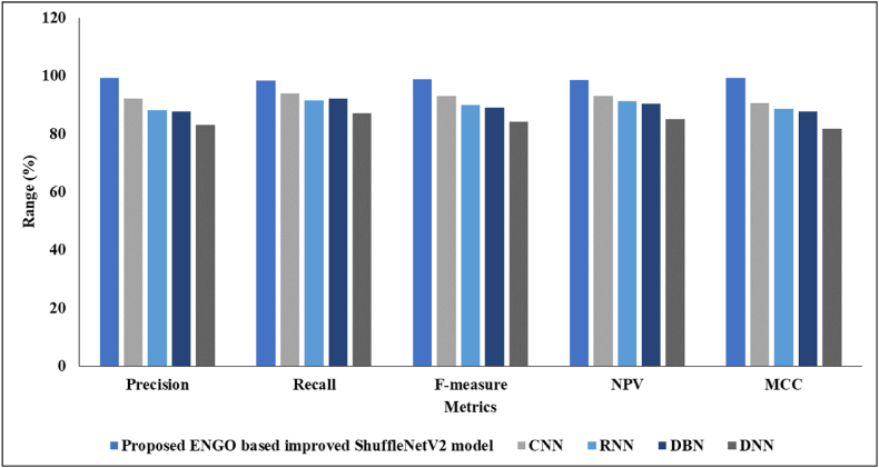
Table 7 presents a comparison of the performance metrics, including Precision, Recall, F-measure, Negative Predictive Value (NPV), and Matthews Correlation Coefficient (MCC), between the current and suggested approaches.
Table 7.
Analysing performance in terms of NPV, MCC, F-measure, Precision, and Recall.
| Methods | Precision | Recall | F-measure | NPV | MCC |
|---|---|---|---|---|---|
| Proposed ENGO based improved ShuffleNetV2 model | 99.1901 | 98.2887 | 98.71357 | 98.5288 | 99.1513 |
| CNN | 92.1416 | 93.9206 | 93.01286 | 92.9929 | 90.6088 |
| RNN | 88.1123 | 91.5453 | 89.9113 | 91.1786 | 88.63026 |
| DBN | 87.7735 | 92.0685 | 89.0158 | 90.3754 | 87.8022 |
| DNN | 83.0583 | 87.1153 | 84.3143 | 85.2012 | 81.7259 |
Table 7 and Fig. 7 provide a comprehensive performance analysis, evaluating different methods based on Precision, Recall, F-measure, Negative Predictive Value (NPV), and Matthews Correlation Coefficient (MCC). The proposed Enhanced Northern Goshawk Optimization (ENGO)-based improved ShuffleNetV2 model demonstrates remarkable precision at 99.19 %, showcasing its ability to accurately identify positive examples. With a recall rate of 98.29 %, the model proves its capability to capture the majority of true positive instances. The F-measure, which balances precision and recall, achieves a notable high of 98.71 %. Furthermore, the Negative Predictive Value (NPV) stands at a substantial 98.53 %, confirming the model's effectiveness in correctly identifying negative instances. The Matthews Correlation Coefficient (MCC) reaches an impressive value of 99.15 %, further validating the robustness of the proposed model. In comparison, alternative methods such as the Recurrent Neural Network, Convolutional Neural Network, Deep Neural Network, and Deep Belief Network exhibit varying levels of performance, with the proposed ENGO-based improved ShuffleNetV2 model consistently outperforming them across multiple evaluation metrics.
Fig. 7.
Performance analysis of the proposed ENGO based improved ShuffleNetV2 classification model.
6. Conclusion
In conclusion, this paper introduces a robust two-phase deep learning methodology for detecting and classifying temperate fish in underwater environments. Recognizing the vital role of underwater cameras in marine ecology applications, the proposed method tackles challenges such as noise, illumination variations, and diverse habitats. Utilising the Unsharp Mask Filter (UMF) for image preprocessing enhances data quality, laying the groundwork for improved analysis. The first phase involves an enhanced region-based fully convolutional network (R–FCN) object detection technique, aimed at optimizing accuracy and eliminating misalignments. The subsequent phase integrates the ShuffleNetV2+Squeeze and Excitation (SE) model, referred to as improved ShuffleNetV2, to enhance attention to target areas and refine classification performance. Hyperparameter tuning is facilitated by the Enhanced Northern Goshawk Optimization Algorithm (ENGO), ensuring optimal model configuration.
The improved R–FCN achieves outstanding object detection results, boasting 99.94 % accuracy, 99.58 % precision/recall, and 99.27 % F-measure on the Fish4knowledge dataset. Meanwhile, the ENGO-based improved ShuffleNetV2 exhibits remarkable classification performance with 99.93 % accuracy, 99.19 % precision, 98.29 % recall, and 98.71 % F-measure. These advancements represent a significant stride in automating the process of finding and categorizing fish in temperate zones, thereby facilitating more efficient and accurate marine ecological studies.
Future research endeavours will focus on expanding the scope of the proposed deep learning methodology, exploring its effectiveness in diverse underwater ecosystems, and incorporating real-time processing capabilities to enhance adaptability in marine ecology applications.
Data availability statement
The data that support the findings of this study are available upon reasonable request from the corresponding author.
Ethics approval
The submitted work is original and has not been published elsewhere in any form or language.
Disclosure of potential conflicts of interest
There is no potential conflict of interest.
Research involving human participants and/or animals
NA.
Funding
The authors declare that no funds, grants, or other support were received during the preparation of this manuscript.
Declaration of competing interest
The authors declare that they have no known competing financial interests or personal relationships that could have appeared to influence the work reported in this paper.
Biographies
1. Dr. D. Siri Currently working as Assistant Professor in the Department of CSE, Gokaraju Rangaraju Institute of Engineering and Technology, Bachupally, TS, India and obtained her B.Tech in Information Technology from JNTU, Hyderabad, M.Tech in Computer Science and Engineering from JNTUH, Hyderabad and Ph.D from JJT University Rajasthan. She published 2 papers in international journals and 1 paper in national and international conferences. Her area of interests are Machine Learning, Software Engineering and IOT
2. Vellaturi Gopikrishna is a Research Scholar at Saveetha institute of medical and technical science, TamilNadu in the area of Machine Learning. Presently he is working as Assistant Professor in the department of IT at MLR institute of Technology, Hyderabad, Telangana. He received his B.Tech. in Computer Science and Engineering from JNTU, Hyderabad and M.Tech in Computer Science and Engineering from JNTU, Ananthapuramu.

3. Dr. Shaik Hussain Shaik Ibrahim, is currently working as an Associate Professor in the Department of Computer Science and Engineering, School of Engineering, Malla Reddy University, Hyderabad, Telangana, India. He received his Bachelor‟s degree in Information Technology from Anna University Coimbatore, TamilNadu, India in 2011, Master‟s degree in Computer Science and Engineering from Anna University, Chennai, TamilNadu, India in 2015 and Ph.D degree in Computer Science and Engineering from Anna University, Chennai, TamilNadu, India in 2020. He has 7 years of teaching and 5 years of research experience including teaching. Also he has 3 years of industry experience. He published 10 papers in SCI and Scopus indexed journals, 7 papers in International Conference and 2 papers in National Conference. He has filed 2 patents and published 1 book. He attended many conferences, seminars, FDPs and workshops in different fields of Computer Science and Engineering. His research area includes Data Mining, Machine Learning, Data Science, Bio Informatics and Bio-Inspired Optimization Algorithms.
4. Srikanth Molugu is an assistant professor at Mallareddy University, specializing in AI and Robotics. He completed his Masters from Andhra University and his Bachelors from Vishnu Institute of Technology. With a passion for innovative ideas, Srikanth has several notable publications to his name in his field of expertise. When he is not teaching or researching, he enjoys exploring new concepts and pushing the boundaries of technology. Srikanth's dedication to his work and his love for exploring new ideas make him a valuable contributor to the field of AI and Robotics.
5. Dr. Venkata Subbaiah Desanamukula received his PhD from Andhra University Visakhapatnam, Under Visvesvaraya Ph.D Scheme Supported by Ministry of electronics and Information Technology (MeitY), Government of India. The author has completed his B.Tech from Nagarjuna University, Andhra Pradesh, and M.Tech from JNTUK, Kakinada. His main research work focuses on object detection using deep learning, cyber security and Machine learning. He has published research papers in various international journals and attended numerous workshops and conferences during his career.
6. Dr. Raviteja Kocherla, is Working as an Associate Professor in the Department of Computer Science & Engineering in Mallareddy University, Hyderabad, has about 12 + years of Teaching & industrial experience. He received his B.Tech. in Information Technology and M.Tech in Computer Science and Engineering from JNTU Hyderabad and Ph.D degree in Computer Science and Engineering from Presidency University, Bangalore. He is having a good number of research papers indexed in SCI and Scopus in refereed international journals and various international conferences. He has published several text books with national and international publishers. He has national & International patent grants.
7. Ramesh Vatambeti received his B.Tech from Sri Venkateswara University, Tirupati in Computer Science and Engineering and M.Tech in IT and PhD in CSE from Sathyabama University, Chennai. He has around 18 years of teaching experience from reputed Engineering Institutions. He works as Professor in the School of Computer Science and Engineering at VIT-AP University, Amaravati, India. He has published more than 70 papers in refereed journals and conference proceedings. He is the reviewer for several refereed International Journals and acted as Session Chair and technical committee member for several International Conferences held in India and abroad. He has successfully guided 3 P h.D. scholars. His research interests include Computer Networks, Mobile Ad-Hoc and Sensor Networks and Machine Learning.
Contributor Information
Siri D, Email: dharmapuri.siri@gmail.com.
Gopikrishna Vellaturi, Email: vellaturigopi@gmail.com.
Shaik Hussain Shaik Ibrahim, Email: shaikhussain2207@gmail.com.
Srikanth Molugu, Email: krishnasrikanth.molugu@gmail.com.
Venkata Subbaiah Desanamukula, Email: desanamukula@gmail.com.
Raviteja Kocherla, Email: tejakcse@gmail.com.
Ramesh Vatambeti, Email: v2ramesh634@gmail.com.
References
- 1.Ditria E.M., Lopez-Marcano S., Sievers M., Jinks E.L., Brown C.J., Connolly R.M. Automating the analysis of fish abundance using object detection: optimizing animal ecology with deep learning. Front. Mar. Sci. 2020;7:429. [Google Scholar]
- 2.Jalal A., Salman A., Mian A., Shortis M., Shafait F. Fish detection and species classification in underwater environments using deep learning with temporal information. Ecol. Inf. 2020;57 [Google Scholar]
- 3.Cui S., Zhou Y., Wang Y., Zhai L. Fish detection using deep learning. Applied Computational Intelligence and Soft Computing. 2020;2020:1–13. [Google Scholar]
- 4.Salman A., Siddiqui S.A., Shafait F., Mian A., Shortis M.R., Khurshid K.…Schwanecke U. Automatic fish detection in underwater videos by a deep neural network-based hybrid motion learning system. ICES (Int. Counc. Explor. Sea) J. Mar. Sci. 2020;77(4):1295–1307. [Google Scholar]
- 5.Ditria E.M., Sievers M., Lopez-Marcano S., Jinks E.L., Connolly R.M. Deep learning for automated analysis of fish abundance: the benefits of training across multiple habitats. Environ. Monit. Assess. 2020;192:1–8. doi: 10.1007/s10661-020-08653-z. [DOI] [PubMed] [Google Scholar]
- 6.Hu J., Zhao D., Zhang Y., Zhou C., Chen W. Real-time nondestructive fish behavior detecting in mixed polyculture system using deep-learning and low-cost devices. Expert Syst. Appl. 2021;178 [Google Scholar]
- 7.Alshdaifat N.F.F., Talib A.Z., Osman M.A. Improved deep learning framework for fish segmentation in underwater videos. Ecol. Inf. 2020;59 [Google Scholar]
- 8.Taheri-Garavand A., Nasiri A., Banan A., Zhang Y.D. Smart deep learning-based approach for non-destructive freshness diagnosis of common carp fish. J. Food Eng. 2020;278 [Google Scholar]
- 9.Akgül T., Calik N., Toreyin B.U. Deep learning-based fish detection in turbid underwater images. IEEE Access. 2020, October;8:1–4. [Google Scholar]
- 10.Al Duhayyim M., Alshahrani H.M., Al-Wesabi F.N., Alamgeer M., Hilal A.M., Hamza M.A. Intelligent deep learning based automated fish detection model for UWSN. CMC-COMPUTERS MATERIALS & CONTINUA. 2022;70(3):5871–5887. [Google Scholar]
- 11.Lisani J.L., Petro A.B., Sbert C., Alvarez-Ellacuria A., Catalan I.A., Palmer M. Analysis of underwater image processing methods for annotation in deep learning based fish detection. IEEE Access. 2022;10:130359–130372. [Google Scholar]
- 12.Chhabra H.S., Srivastava A.K., Nijhawan R. Proceedings of ICETIT 2019: Emerging Trends in Information Technology. Springer International Publishing; 2020. A hybrid deep learning approach for automatic fish classification; pp. 427–436. [Google Scholar]
- 13.Allken V., Rosen S., Handegard N.O., Malde K. A deep learning-based method to identify and count pelagic and mesopelagic fishes from trawl camera images. ICES (Int. Counc. Explor. Sea) J. Mar. Sci. 2021;78(10):3780–3792. [Google Scholar]
- 14.Abinaya N.S., Susan D., Sidharthan R.K. Deep learning-based segmental analysis of fish for biomass estimation in an occulted environment. Comput. Electron. Agric. 2022;197 [Google Scholar]
- 15.Ahmed M.S., Aurpa T.T., Azad M.A.K. Fish disease detection using image based machine learning technique in aquaculture. Journal of King Saud University-Computer and Information Sciences. 2022;34(8):5170–5182. [Google Scholar]
- 16.Wang G., Muhammad A., Liu C., Du L., Li D. Automatic recognition of fish behavior with a fusion of RGB and optical flow data based on deep learning. Animals. 2021;11(10):2774. doi: 10.3390/ani11102774. [DOI] [PMC free article] [PubMed] [Google Scholar]
- 17.Pezoa J.E., Ramírez D.A., Godoy C.A., Saavedra M.F., Restrepo S.E., Coelho-Caro P.A.…Urbina M.A. A spatial-spectral classification method based on deep learning for controlling pelagic fish landings in Chile. Sensors. 2023;23(21):8909. doi: 10.3390/s23218909. [DOI] [PMC free article] [PubMed] [Google Scholar]
- 18.Liu H., Ma X., Yu Y., Wang L., Hao L. Application of deep learning-based object detection techniques in fish aquaculture: a review. J. Mar. Sci. Eng. 2023;11(4):867. [Google Scholar]
- 19.López-Barajas S., Sanz P.J., Marín-Prades R., Gómez-Espinosa A., González-García J., Echagüe J. Inspection operations and hole detection in fish net cages through a hybrid underwater intervention system using deep learning techniques. J. Mar. Sci. Eng. 2023;12(1):80. [Google Scholar]
- 20.Silva C.N., Dainys J., Simmons S., Vienožinskis V., Audzijonyte A. A scalable open-source framework for machine learning-based image collection, annotation and classification: a case study for automatic fish species identification. Sustainability. 2022;14(21) [Google Scholar]
- 21.Zhang S., Yang X., Wang Y., Zhao Z., Liu J., Liu Y.…Zhou C. Automatic fish population counting by machine vision and a hybrid deep neural network model. Animals. 2020;10(2):364. doi: 10.3390/ani10020364. [DOI] [PMC free article] [PubMed] [Google Scholar]
- 22.Martin-Abadal M., Ruiz-Frau A., Hinz H., Gonzalez-Cid Y. Jellytoring: real-time jellyfish monitoring based on deep learning object detection. Sensors. 2020;20(6):1708. doi: 10.3390/s20061708. [DOI] [PMC free article] [PubMed] [Google Scholar]
- 23.Er M.J., Chen J., Zhang Y., Gao W. Research challenges, recent advances, and popular datasets in deep learning-based underwater marine object detection: a review. Sensors. 2023;23(4):1990. doi: 10.3390/s23041990. [DOI] [PMC free article] [PubMed] [Google Scholar]
- 24.Chen Y., Ling Y., Zhang L. Accurate fish detection under marine background noise based on the retinex enhancement algorithm and CNN. J. Mar. Sci. Eng. 2022;10(7):878. [Google Scholar]
- 25.Ben Tamou A., Benzinou A., Nasreddine K. Live fish species classification in underwater images by using convolutional neural networks based on incremental learning with knowledge distillation loss. Machine Learning and Knowledge Extraction. 2022;4(3):753–767. [Google Scholar]
- 26.Li E., Wang Q., Zhang J., Zhang W., Mo H., Wu Y. Fish detection under occlusion using modified You only look once v8 integrating real-time detection transformer features. Appl. Sci. 2023;13(23) [Google Scholar]
- 27.Kuswantori A., Suesut T., Tangsrirat W., Schleining G., Nunak N. Fish detection and classification for automatic sorting system with an optimized YOLO algorithm. Appl. Sci. 2023;13(6):3812. [Google Scholar]
- 28.Wang Z., Liu H., Zhang G., Yang X., Wen L., Zhao W. Diseased fish detection in the underwater environment using an improved YOLOV5 network for intensive aquaculture. Fishes. 2023;8(3):169. [Google Scholar]
- 29.Ranjan R., Tsukuda S., Good C. Effects of image data quality on a convolutional neural network trained in-tank fish detection model for recirculating aquaculture systems. Comput. Electron. Agric. 2023;205 [Google Scholar]
- 30.Fernandez Garcia G., Corpetti T., Nevoux M., Beaulaton L., Martignac F. AcousticIA, a deep neural network for multi-species fish detection using multiple models of acoustic cameras. Aquat. Ecol. 2023:1–13. [Google Scholar]
- 31.Patro K.S.K., Yadav V.K., Bharti V.S., Sharma A., Sharma A. Fish detection in underwater environments using deep learning. Natl. Acad. Sci. Lett. 2023;1–6 [Google Scholar]
- 32.Lin Y., Chu Z., Korhonen J., Xu J., Liu X., Liu J.…You J. International Conference on Multimedia Modeling. Springer International Publishing; Cham: 2023, January. Fast accurate fish recognition with deep learning based on a domain-specific large-scale fish dataset; pp. 515–526. [Google Scholar]
- 33.Kandimalla V., Richard M., Smith F., Quirion J., Torgo L., Whidden C. Automated detection, classification and counting of fish in fish passages with deep learning. Front. Mar. Sci. 2022;8:2049. [Google Scholar]
- 34.Al Muksit A., Hasan F., Emon M.F.H.B., Haque M.R., Anwary A.R., Shatabda S. YOLO-Fish: a robust fish detection model to detect fish in realistic underwater environment. Ecol. Inf. 2022;72 [Google Scholar]
- 35.Alaba S.Y., Nabi M.M., Shah C., Prior J., Campbell M.D., Wallace F.…Moorhead R. Class-aware fish species recognition using deep learning for an imbalanced dataset. Sensors. 2022;22(21):8268. doi: 10.3390/s22218268. [DOI] [PMC free article] [PubMed] [Google Scholar]
- 36.Hong Khai T., Abdullah S.N.H.S., Hasan M.K., Tarmizi A. Underwater fish detection and counting using mask regional convolutional neural network. Water. 2022;14(2):222. [Google Scholar]
- 37.Yin J., Wu J., Gao C., Yu H., Liu L., Jiang Z., Guo S. Individual fish recognition method with coarse and fine-grained feature linkage learning for precision aquaculture. Aquacult. Res. 2023;2023 [Google Scholar]
- 38.Knausgård K.M., Wiklund A., Sørdalen T.K., Halvorsen K.T., Kleiven A.R., Jiao L., Goodwin M. Temperate fish detection and classification: a deep learning-based approach. Appl. Intell. 2022:1–14. [Google Scholar]
- 39.Zheng L., Xu W. An improved adaptive spatial preprocessing method for remote sensing images. Sensors. 2021;21(17):5684. doi: 10.3390/s21175684. [DOI] [PMC free article] [PubMed] [Google Scholar]
- 40.Zhang D., Li F., Ding X., Sangaiah A.K., Sheng V.S. Small object detection via precise region-based fully convolutional networks. Comput. Mater. Continua (CMC) 2021;69(2) [Google Scholar]
- 41.Xu X., Zhang Y., Cao H., Yang D., Zhou L., Yu H. Recognition of edible fungi fruit body diseases based on improved ShuffleNetV2. Agronomy. 2023;13(6):1530. [Google Scholar]
- 42.Liang Y., Hu X., Hu G., Dou W. An enhanced northern goshawk optimization algorithm and its application in practical optimization problems. Mathematics. 2022;10(22):4383. [Google Scholar]
Associated Data
This section collects any data citations, data availability statements, or supplementary materials included in this article.
Data Availability Statement
The data that support the findings of this study are available upon reasonable request from the corresponding author.


