A General Bayesian Functional Spatial Partitioning Method for Multiple Region Discovery Applied to Prostate Cancer MRI

Abstract

Current protocols to estimate the number, size, and location of cancerous lesions in the prostate using multiparametric magnetic resonance imaging (mpMRI) are highly dependent on reader experience and expertise. Automatic voxel-wise cancer classifiers do not directly provide estimates of number, location, and size of cancerous lesions that are clinically important. Existing spatial partitioning methods estimate linear or piecewise-linear boundaries separating regions of local stationarity in spatially registered data and are inadequate for the application of lesion detection. Frequentist segmentation and clustering methods often require pre-specification of the number of clusters and do not quantify uncertainty. Previously, we developed a novel Bayesian functional spatial partitioning method to estimate the boundary surrounding a single cancerous lesion using data derived from mpMRI. We propose a Bayesian functional spatial partitioning method for multiple lesion detection with an unknown number of lesions. Our method utilizes functional estimation to model the smooth boundary curves surrounding each cancerous lesion. In a Reversible Jump Markov Chain Monte Carlo (RJ-MCMC) framework, we develop novel jump steps to jointly estimate and quantify uncertainty in the number of lesions, their boundaries, and the spatial parameters in each lesion. Through simulation we show that our method is robust to the shape of the lesions, number of lesions, and region-specific spatial processes. We illustrate our method through the detection of prostate cancer lesions using MRI.

1. Introduction

Multiparametric magnetic resonance imaging (mpMRI), a combination of MRI images, has improved diagnostic accuracy for detecting prostate cancer compared to previous methods (Ahmed et al., 2017). Computer-aided diagnostic (CAD) systems to estimate voxel-wise cancer probabilities based on mpMRI features continue to be developed and evaluated (Fei, 2017). Previously, our group developed fully automated voxel-wise classifiers that account for regional heterogeneity in the prostate and spatial dependence in the data without the need for manual segmentation (Jin et al., 2018, 2022). While these models can guide clinicians in locating approximate areas with high probability of cancer, an additional step to translate probabilities into lesions is needed for use in clinical practice. Besides estimating location and size, correctly identifying the number of cancerous lesions is important, clinically (Leng et al., 2018).

Previously we developed Bayesian Functional Spatial Partitioning, re-named as BFSP-1, a boundary detection method for spatially correlated data exhibiting a single anomalous region (Masotti et al., 2021). This method proved to be successful when applied to data derived from mpMRI containing a single cancerous lesion. However, BFSP-1 is not applicable when the data have zero or more than one anomalous regions, which is common in practice. As we show in our simulations, BFSP-1 may detect one or more separate anomalous regions with a single partitioning boundary. This precludes applying BFSP-1 repeatedly to one imaging slice containing multiple anomalous regions. Further, we aim to estimate the uncertainty in both the number and location of lesion boundaries, which BFSP-1 cannot do.

Estimating the true number of distinct groups, clusters, or lesions in a spatially referenced dataset is a challenging and largely unsolved problem in frequentist statistics. Existing methods for estimating the true number of clusters tend to be ad-hoc or require unrealistic assumptions and complicated calculations (Sugar and James, 2003; Salvador and Chan, 2004; Jain, 2010). Determining the optimal number of terminal nodes or partitions in a decision tree is similarly challenging. Classification and regression trees (CART) (Breiman et al., 1984) recursively split the data until no additional split improves the homogeneity within the nodes. CART tends to overestimate the number of nodes and often requires ad-hoc pruning methods to prevent over-fitting (Denison et al., 1998). Clustering methods using likelihood maximization do not provide estimates of uncertainty in the number of clusters or cluster membership.

Bayesian modeling provides a straightforward framework for estimating the number of clusters and the uncertainty of the estimate. This is typically accomplished using Bayesian mixture models that estimate voxel-wise cluster membership (Fruhwirth-Schnatter et al., 2019; Argiento and De Iorio, 2022; Neal, 2000). Product partition models, first introduced by Hartigan (1990), create clusters using a prior that takes the form of a product of cohesion functions. The cohesion function measures how likely data points are to be clustered together. Page and Quintana (2016) develops a spatial version of the product partition model by making the cohesion a function of spatial location. The method by Teixeira et al. (2019) extends the PPM to the spatio-temporal context. PPMs are constructed to find clusters. When data exhibit homogenity (data belong to one cluster), PPMs are not appropriate. For this reason, PPMs are not appropriate for our data as a healthy individual’s imaging data would in theory contain no clusters. Kang et al. (2018) developed a soft-thresholded Gaussian process model to partition the brain in order to detect regions that are highly predictive of alcoholism using EEG data. This regression method detects spatial regions that are important on average across several patients and time points. We aim to detect distinct regions from each patient’s imaging data. None of the above methods provide estimates of boundaries or boundary uncertainty, which are of critical importance to our clinicians.

Bayesian random partitioning models can quantify uncertainty in the number and locations of boundaries but existing methods are not well suited for our application. Denison et al. (1998) developed a Bayesian CART algorithm which provides insight into a range of good trees of varying depth rather than returning a point estimate. Denison and Holmes (2001) developed a Bayesian partition model for count data based on a Voronoi tessellation in which centroids are proposed and data points are assigned to the nearest center. Chipman et al. (2002) extended the Bayesian CART method by fitting hierarchical linear models in each terminal node. The spatial partitioning methods by Gramacy and Lee (2008) and Konomi et al. (2014) fit Gaussian processes (GPs) in the terminal nodes. The method by Kim et al. (2005) also uses Voronoi tessellation in which the tiles follow distinct GPs. However, all of the above methods assume linear or piece-wise linear partitioning boundaries. Prostate cancer lesions can be of any shape, rendering these methods inadequate for our application. The Bayesian regularization method by Lee et al. (2021) estimates partitions of data whose prior structure is represented by a graph. The proposed linear model does not include spatial random error, which our data clearly exhibits.

Our goal is to develop a fully automated lesion detection pipeline that jointly estimates the number of lesions and their boundaries from a patient’s mpMRI data using a Bayesian approach. This allows quantification of uncertainty in both the number of lesions and their boundaries. We propose BFSP-M, a general framework to identify and describe an unknown number of arbitrarily shaped anomalous regions using boundary detection for spatially registered data. BFSP-M uses separate moving polar systems for each lesion, within which the boundary curves are estimated via functional approximation, and reversible jump Markov chain Monte Carlo (RJ-MCMC) to explore parameter spaces of different dimensions which vary with the number of lesions. In the same vein as Richardson and Green (1997), we develop four jump steps to add, subtract, split, and merge the lesion-defining boundaries. Richardson and Green (1997) uses jump proposals to add or subtract densities in a mixture model, while our method defines proposals to add or subtract boundaries and updates the corresponding boundary parameters. These moves efficiently avoid the local-trap problem in our Bayesian spatial partitioning and ensure faster mixing and convergence in estimating the number of lesions. Compared to machine learning methods for imaging segmentation, our method allows estimation of uncertainty as to the number of lesions and each lesion boundary. While the proposed model is intended for single patient and single slice analysis, our method provides a statistical modeling framework that allows extensions to multi-slice, multi-subject, and/or longitudinal analysis of lesion status which we will discuss in more detail in Section 7. We show through simulations that BFSP-M can detect multiple irregularly shaped regions with higher sensitivity and specificity compared to competing image segmentation methods. An application to the data from Metzger et al. (2016) and Jin et al. (2018) illustrates the flexibility to identify an unknown number of cancerous lesions of arbitrary shape in the prostate using mpMRI. While our application is specific, this method of partitioning is general and can be applied to any type of spatially related data that contains anomalous areas within a larger homogeneous space.

The remainder of the paper is organized as follows. We introduce our novel Bayesian model for functional spatial partitioning and discuss Bayesian modeling of the underlying spatial process in Section 2. We discuss the computational implementation of our method via RJ-MCMC in Section 3. In Section 4 we develop a post-processing procedure and estimate credibility bands for the boundaries. We evaluate the statistical properties of our method via simulation and compare its performance to existing methods in Section 5. This is followed by an application to the data from Jin et al. (2018) in Section 6. Finally, we conclude with a discussion and suggest future extensions in Section 7.

2. Model Specification

Our objective is to estimate the set of boundaries $\left\{B_1,\dots ,B_m\right\}$ that partitions the data into multiple regions based on heterogeneity in the underlying spatial processes with minimal restrictions on the shapes of the target regions. The model is specified by three components. First, we model the set of boundaries as functions of angles with respect to a set of centroids. Second, we specify the likelihood for the data though a piecewise spatial Gaussian process conditional on the partition generated by the set of boundaries. Finally, we assign priors for all the parameters to complete the full Bayesian model. Estimation is accomplished iteratively via RJ-MCMC to jointly estimate the number of target regions, the boundary parameters, and the spatial parameters based on their posterior probabilities given the data.

Section 2.1 discusses how a partition with $m$ boundaries is defined by a set of boundaries, $B_1,\dots ,B_m$. In Section 2.2, we specify the likelihood. The full hierarchical mode as well as details on the prior are provided in Section 2.3. Finally, details of Bayesian computations are given in Section 3.

2.1. Defining a Partition

Let $Z\left(s\right)$ indicate a scalar variable that is observed at location $s=\left(x,y\right)\in D$, where $D$ is a region in $R^2$. In our application, we assume $D$ to be a unit square. Let $\mathit{s}=$ $\left(s_1,\dots s_n\right)$ and $\mathit{Z}=\left(Z\left(s_1\right),\dots ,Z\left(s_n\right)\right)$ denote a set of locations within the region $D$ and the corresponding set of observations. Assume some partition of the space with $m\ge 0$ mutually exclusive contiguous regions, $D_1,\dots ,D_m$, all within $D$, defined by boundaries $B_1,\dots ,B_m$ and $D_0=D\setminus D_1\setminus \cdots \setminus D_m$. Let ${\mathit{s}}_j$ be the vector of spatial locations within region $D_j$ and ${\mathit{Z}}_j$ the vector of observed values at those locations. We assume each vector ${\mathit{Z}}_j$ follows a distinct distribution.

A partition of $D$ with $m$ boundaries $B_1,\dots ,B_m$ creates $m+1$ regions $D_0,D_1,\dots ,D_m$ In our motivating problem, $D_0$ represents the healthy tissue and regions $D_1,\dots ,D_m$ represent $m$ non-overlapping cancerous regions. Given a point $c_j$ located at the centroid of $D_j$, the boundary curve $B_j$ can be uniquely modeled as a function of an angle in a polar coordinate system centered at $c_j$. We define the boundary $B_j=\{s\in D:d_{c_j\to s}=$$f_j\left({\theta }_s\mid c_j,{\mathit{\beta }}_j\right),{\theta }_s\in \left[0,2\pi \right]\}$, where $d_{c\to s}$ is the distance between a point $\mathit{s}$ and the polar center $c,{\theta }_s$ is the angle formed between the line connecting $c_j$ and $s$ and the horizontal, and ${\mathit{\beta }}_j$ are parameters defining the boundary function. Thus modeling the boundary curves is equivalent to estimating the locations of the $c_j$ and the functions $f_j\left(\theta \mid c_j,{\mathit{\beta }}_j\right)$ for $j=1,\dots ,m$. Each spatial location $s$ can be assigned to a region by its distance $d_{c_j}\left(s\right)$ referenced to the centroids $c_j$ for $j=1,\dots ,m$. See Figure 1 for an illustration of our partitioning method.

Figure 1:

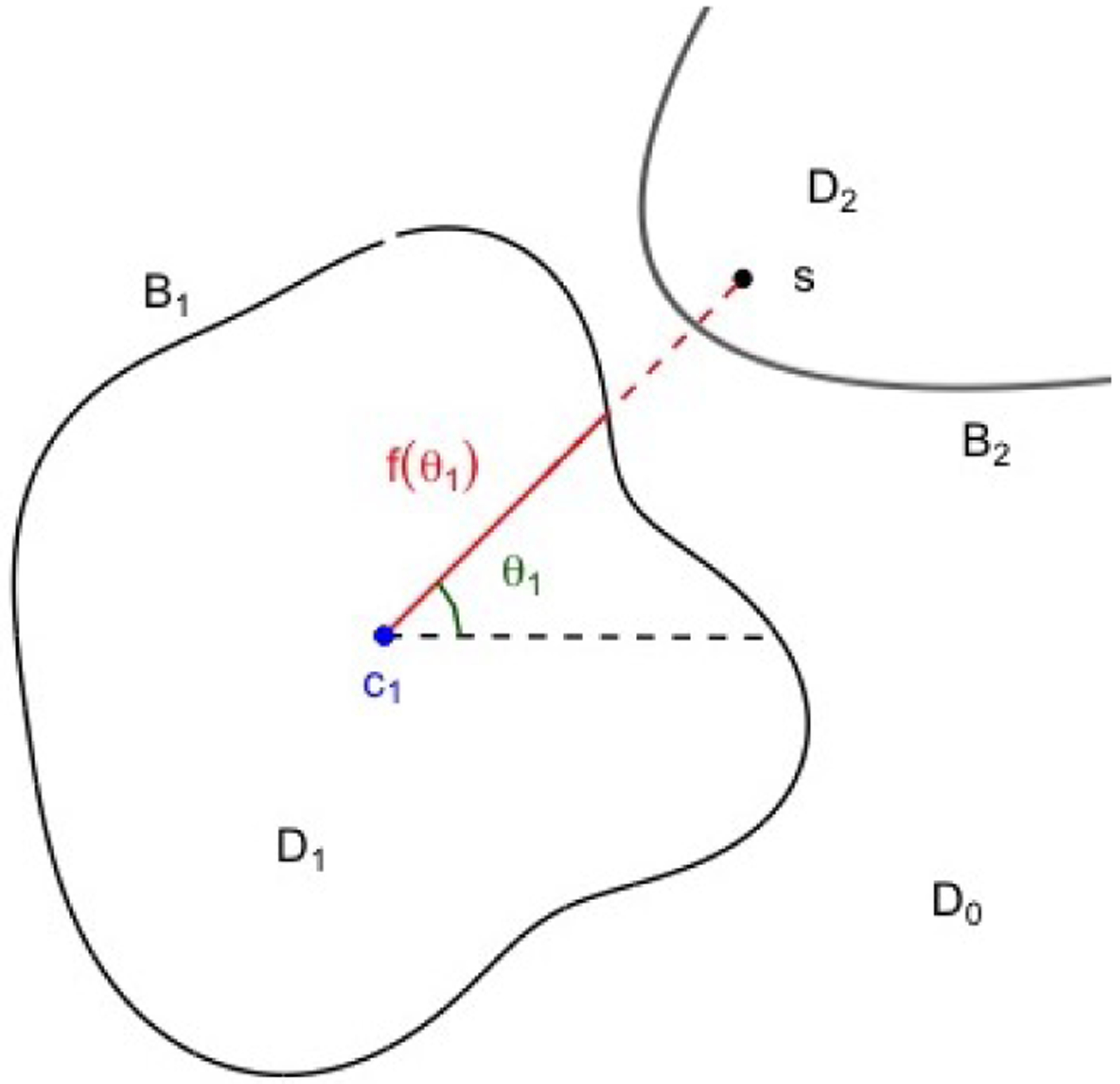
An example of how spatial locations are assigned given multiple boundaries. Boundaries $B_1$ and $B_2$ are shown in black. $s=\left(x,y\right)$ is a spatial location, $c_1$ is the centroid of $B_1$ at the current iteration, ${\theta }_1$ is the angle between the horizontal and the line from $s$ and $c_1$, and $f\left({\theta }_1\right)$ is the magnitude of the boundary at ${\theta }_1$. In this example, $s$ is categorized as within region $D_2$ but not $D_1$ : the distance from $s$ to $c_1$ is greater than $f\left({\theta }_1\right)$.

The boundary functions are estimated by a linear combination of $\text{K}$ basis functions. The only constraint on the choice of basis function is that they must be periodic ensuring $f\left(0\right)=f\left(2\pi \right)$. In our previous work we show that Fourier and spline basis functions work well for our application (Masotti et al., 2021). The boundary function implemented with Fourier basis functions takes this form:

$$f_j\left({\theta }_a\mid c_j,{\mathit{\beta }}_j\right)={\beta }_{j,0}+\sum _{k=1}^K{\beta }_{j,k}^s\text{sin}\left(k{\theta }_s\right)+{\beta }_{j,k}^c\text{cos}\left(k{\theta }_s\right)\text{for}0\le {\theta }_s\le 2\pi$$ (1)

where ${\beta }^s$ and ${\beta }^c$ indicate coefficients corresponding to the sine and cosine basis functions, respectively, and ${\mathit{\beta }}_j=\left({\beta }_{j,0},{\beta }_{j,K}^s,\dots ,{\beta }_{j,K}^z,{\beta }_{j,1}^c,\dots ,{\beta }_{j,K}^c\right)$. While we use Fourier and spline basis functions for lesion detection, wavelets can also be used to model bumpy boundary functions as long as they satisfy the constraint. For the simulation and data analysis, we implement our method with Fourier basis functions. Note that by modeling boundaries as functions of angles, our method is restricted to boundary estimation in the star domain. A region $S$ is in the star domain if there exists an $x_0$ in $\text{S}$ such that for all $x$ in $\text{S}$ the line segment from $x_0$ to $x$ is in $S$. That is, our method cannot estimate boundary curves with radial concavities. However, for our motivating application, a lesion exhibiting radial concavity could be captured by two or more neighboring boundaries that achieve the same goal clinically. The parameter $K$ corresponds to the level of detail in the boundary. A lower value will produce a smoother boundary. In our previous work we found that $K=5$ was adequate for lesion detection in our data. However for other applications, the value of $K$ can be treated as an additional parameter and chosen by cross-validation by the user.

2.2. Spatial Modeling

We now consider the likelihood via spatial modeling of the data conditional on the spatial partition given above. Estimation of the spatial process within each region occurs simultaneously with estimation of the boundary. At each iteration, by transitioning back into Cartesian coordinates we can classify a spatial location $s$ as within region $D_j$ if $s$ is within the boundary, i.e., the distance $d_{c_j\to s}$ is less than the boundary function (1) at ${\theta }_{c_f}\left(s\right)$. Given a current estimate of $m$ regions with centroids $c_j$ and boundary functions $f_{c_j}(·)$ for $j=1,\dots ,m$, we can partition the space into $D_j=\{s\in D:d_{c_j\to s}\le f_j\left({\theta }_s\mid {\varphi }_j\right),{\theta }_s\in [0,2\pi )\}$ and $D_0=\left\{s\in D:s\notin D_j\forall j=1,\dots ,m\right\}$. Let ${\mathit{s}}_j$ be the vector of spatial locations within region $D_j$ and ${\mathit{Z}}_j$ the vector of observed values at those locations. Let ${\mathbf{\Phi }}_m=\left({\varphi }_0,{\varphi }_1,\dots ,{\varphi }_m\right)$ be all of the parameters describing a given partition where ${\varphi }_0$ contains the parameters which define the Gaussian spatial process of data contained in $D_0$ and ${\varphi }_j$ contains the parameters which define the Gaussian spatial process of data contained in $D_j$ and the parameters defining the boundary $B_j$. For a given partition of the data with $m$ boundaries, we assume the data from different regions are conditionally independent and follow a piecewise Gaussian spatial process. That is, we can calculate the likelihood as the product of $m+1$ independent likelihoods:

$$L\left(\mathit{Z}\mid m,{\mathbf{\text{Φ}}}_m\right)={\prod }_{j=0}^{m}L\left({\mathit{Z}}_j\mid {\varphi }_j\right).$$ (2)

In each region we assume a distinct stationary Gaussian spatial process. Marginalizing over the spatial effects, the distribution of the data $Z_j$ in region $j$ or $j=0,\dots ,m$ is given by:

$$\begin{gathered} {\mathit{Z}}_j\mid {\varphi }_j~N\left({\mu }_j,{\text{Σ}}_j\right) \\ {\text{Σ}}_j={\sigma }_j^{2}H\left(\gamma \right)+{\tau }^2{I}_{n_j} \end{gathered}$$ (3)

where ${\mu }_j$ is the mean specific to region $j$, and ${\mathit{\xi }}_j$ is the vector of spatial random effects that follow a region-specific Gaussian distribution with covariance ${\sigma }_j^{2}H\left(\gamma \right)$. The variance for non-spatial random errors, ${\tau }^2$, is assumed to be common to all regions.

We encourage spatial smoothness within each region by assuming an exponential kernel.

$$H\left(s_i,s_i^{\text{'}}\mid \gamma \right)=\text{exp}\left(-\gamma d_{i\to i^{\prime }}\right)$$

where $d_{i\to i^{\prime }}$ is the Euclidean distance and $\gamma$ is the spatial decay parameter which is assumed to be common to all regions. Other kernels can be specified. We chose the exponential kernel due to its simplicity and its ability to approximate other types of spatial correlation structures well.

Fitting the likelihood with the spatial model specified in (3) becomes infeasible when $n$ is large due to the time requirements of calculating the determinant and inverse of the covariance matrices. Due to the size of the data in the imaging context, we opt to make two assumptions of the spatial likelihood to facilitate Bayesian computation without detriment to model estimation. Although we note that users in a small data context may opt to use the full likelihood.

First, we divide $D_0$ into four roughly equally sized and independent zones. The mean $x$ and $y$ coordinates of $s\in D_0$ at a given iteration define the boundaries that split the area into $Z_{0,1},\dots ,Z_{0,4}$. Thus, the likelihood in (3) is assumed by:

$$L\left(\mathit{Z}\mid {\mathbf{\text{Φ}}}_m,m\right)\approx {\prod }_{l=1}^{4}L\left({\mathit{Z}}_{0,l}\mid {\varphi }_0\right){\prod }_{j=1}^{m}L\left({\mathit{Z}}_j\mid {\varphi }_j\right)$$

The underlying assumption is that the spatial correlations across these large sub-regions are relatively ignorable and the joint likelihood can be well approximated by independent spatial modeling of each sub-region.

Second, we assume a sparse covariance matrix by multiplying the assumed covariance matrix by a tapering kernel $C_{\nu }\left(s_i,s_{i^{\prime }}\right)$. Tapered covariances are commonly used to analyze large spatial datasets as they allow for sparse matrix algorithms. The tapering kernel must be a positive definite matrix such that the covariance between two spatial locations becomes zero after a given distance. The Wendland family of tapered covariance functions (Wendland, 1995) are widely used. We assume the form of

$$C_{\nu }\left(s_i,s_{i^{\prime }}\right)={\left(1-\frac{h}{\nu }\right)}_{+}^4\left(1+4\frac{h}{\nu }\right),$$

Where $h=\Vert s_i-s_{i^{\prime }}\Vert ,{(y)}_{+}=y{I}_{\{y>0\}}$, and we fix $\nu =.1$. This yields our assumed covariance matrix:

$${\text{Σ}}_j\approx {\sigma }_j^{2}H\left(\gamma \right)\odot T_j+{\tau }^2{I}_{n_j}$$

where $\odot$ denotes the element-wise product, $\text{H}$ is based on the exponential kernel, $T_j$ is the $n_j\times n_j$ matrix with the $\left(i,i^{\prime }\right)$-th entry $C_{\nu }\left(s_i,s_{i^{\prime }}\right)$.

2.3. Bayesian Hierarchical Model

We now assign priors for all the boundary and spatial parameters to complete our Bayesian hierarchical model. First, we present details on the prior. We conclude by presenting the full hierarchical model.

Note that the voxels of all the images we consider in our motivating data are scaled to fall within the unit square. In this case, the prior hyperparameters we specify are universal. Otherwise one can scale the hyperparameter in the priors proportionally with respect to the size of the image. Let $\mathit{\beta }=\left({\mathit{\beta }}_1,\dots ,{\mathit{\beta }}_m\right),\mathit{c}=\left(c_1,\dots ,c_m\right),\mathit{\mu }=\left({\mathit{\mu }}_1,\dots ,{\mathit{\mu }}_m\right)$, and ${\mathit{\sigma }}^2=\left({\mathit{\sigma }}_1^2,\dots ,{\mathit{\sigma }}_m^2\right)$

$$m~\text{DiscreteUnif}\left(m;M_{\text{min}},M_{\text{max}}\right)$$ (4)

$$\mathit{\beta },\mathit{c}~1_{\left\{\mathit{\beta },\mathit{c}\right\}\notin s}\prod _{j=1}^m\frac{1_{c_j\in D}}{\parallel D\parallel }\text{Unif}\left({\beta }_{j,0};0,r\left(D\right)\right)\prod _{k=1}^K\prod _{l\in \left\{s,c\right\}}N\left({\beta }_{j,k}^l;0,1\right)$$ (5)

where $\mathit{𝒮}=\left\{\{\mathit{\beta },\mathit{c}\};\exists s\in D_j\cap D_k,j\ne k\right\}$

$$\mathit{\mu }~N\left({\mu }_0;0,100\right)\prod _{j=1}^{m}HN\left({\mu }_j-{\mu }_0;0,10\right)$$ (6)

$${\mathit{\sigma }}^2~\prod _{j=1}^{m}IG\left({\sigma }_j^2;.1,.1\right),{\tau }^2~IG\left({\tau }^2;.1,.1\right),\gamma ~G\left(\gamma ;3,.5\right)$$ (7)

The number of boundaries $m$ is uniform between some minimum and maximum value set by the user (4). In our simulation and data analysis we use values of 0 and 10, respectively. The centroids are assumed to be uniformly distributed across $D$. We assign normal marginal priors $N\left(0,1\right)$ to all basis coefficients in ${\mathit{\beta }}_j^s$ and ${\beta }_j^c$. This is a vague prior when the area of the entire region is standardized to be a $1\times 1$ unit square. We place a uniform marginal prior on ${\beta }_{j,0}$ from zero to the approximate radius of $D$, denoted $r\left(D\right)$, to ensure that the area within the closed boundary does not greatly exceed the entire space of interest. The first indicator function in (5) places zero mass on combinations of boundary and centroid parameters that would result in a spatial location $s$ being included in more than one boundary. In the MCMC, we simply reject any update or proposal of ${\mathit{\beta }}_j,c_j$ which would lead to overlap of the boundaries. We assign the mean of the outer region a vague normal marginal prior $N\left(0,100\right)$. The difference in means between a target region and the outer region is assumed to follow a vague half-normal marginal prior $HN\left(0,10\right)$ because we have prior information that the mean of the anomalous region is elevated as compared to the rest of the space (6). This can be modified for other applications. Following the advice of Banerjee et al. (2014), we assign vague marginal priors for the variance parameters ${\sigma }^2$ and ${\tau }^2$ and an informative marginal prior for spatial range parameter $\gamma$. Thus $IG\left(.1,.1\right)$ is the marginal prior used for ${\sigma }^2$ and ${\tau }^2$ parameters and the spatial range parameter $\gamma$ follows $G\left(3,.5\right)$ (7).

Again, let ${\mathbf{\Phi }}_m=\left({\varphi }_0,{\varphi }_1,\dots ,{\varphi }_m\right)$ be all of the parameters describing a given partition where ${\varphi }_0=\left({\mu }_0,{\sigma }_0^2,{\tau }^2\right)$ and ${\varphi }_j=\left({\mu }_j,{\sigma }_j^2,{\mathit{\beta }}_j,c_j\right)$ for $j=1,\dots ,m$. The full hierarchical model is given by:

$$\pi \left(m,{\mathbf{\text{Φ}}}_m\mid \mathit{Z}\right)\propto L\left(\mathit{Z}\mid m,{\mathbf{\text{Φ}}}_m\right)\pi \left({\mathbf{\text{Φ}}}_m\mid m\right)\pi \left(m\right)$$ (8)

where $\pi \left({\mathbf{\text{Φ}}}_m\mid m\right)\pi \left(m\right)$ is the joint prior of (4)-(7) above. From (2)-(3):

$$\begin{gathered} \pi \left(Z\mid m,{\Phi }_m\right)=\prod _{j=0}^m\pi \left(Z_j\mid {\varphi }_j\right),\text{where}{Z}_j=Z\left({\mathit{s}}_j\right),{\mathit{s}}_j=\left\{s\in \mathit{s}:s\in D_j\right\} \\ {D}_j\mid {\varphi }_j=\left\{s\in D:d_{s\to c_j}<f_j\left({\theta }_s\mid {\varphi }_j\right)\right\},D_0=D/{\left\{D_j\right\}}_{j=1,\dots ,m} \\ {\mathit{Z}}_0\mid {\varphi }_0~\prod _{l=1}^{4}N\left(Z_{0,l}\mid {\mu }_0,{\tau }^{2}I+{\sigma }_0^{2}H(\gamma )\odot T_{0,l}\right) \\ {\mathit{Z}}_j\mid {\varphi }_j~N\left(Z_j;{\mu }_j,{\tau }^{2}I+{\sigma }_j^{2}H(\gamma )\odot T_j\right) \end{gathered}$$ (9)

3. Bayesian Computation via RJ-MCMC

We propose a schema to jointly estimate the number of target regions, the boundary parameters, and the spatial parameters based on their posterior probabilities given the data. During the MCMC, the number of bonudaries will not be fixed, therefore the total number of parameters is also not fixed. This necessitates the use of RJ-MCMC to allow the MCMC chain to jump between parameter spaces of different dimensions, The RJ-MCMC algorithm by Green (1995) is an extension of the Metropolis Hastings (MH) algorithm that allows movement between different dimensional spaces. In the RJ-MCMC, we propose addition, deletion, splitting, and merging of boundaries and corresponding lesions to allow the chain to move between different partitions. We refer to the addition of a new boundary as a “birth”, the deletion of an existing boundary as a “death”. We also introduce the merging of two existing boundaries as a “merge”, and the splitting of one existing boundary into two as a “split”. The “split” and “merge” types of jump efficiently prevent the MCMC chain from being trapped in local minima and thus greatly speed up mixing and convergence of spatial partitions. With a specified probability, a birth, death, split, or merge is proposed and the current boundary and distribution parameters are updated. Moves are automatically rejected if they lead to overlapping boundaries. Adaptive MH is used to update the boundary and GP parameters given the current number of regions.

Let $m$ be the current number of regions and $m^{\prime }$ the proposed number of boundaries, which are both between $M_{\text{min}}$ and $M_{\text{max}}$. We allow movements that increase or decrease the number of regions by one at each iteration. The RJ-MCMC algorithm is composed of two steps: 1. propose a new partition with corresponding parameters, and 2. calculate the acceptance ratio to determine whether to accept or reject the proposed move. RJ-CMC uses two types of proposal distributions.

• $j\left(m^{\prime }\mid m\right)$ is the model proposal. It defines the probability of switching from $m$ to $m^{\prime }$ boundaries and must be reversible.

• $q\left(\mathbf{v}\right)$ is the auxiliary variable proposal distribution where $\mathbf{v}$ is used to match dimension between $m$ and $m\text{'}$.

RJ-MCMC also requires a mapping function $h_{m,m^{\prime }}\left({\Phi }_m,v\right)$ which maps $\left({\Phi }_m,v\right)$ to $\left({\mathbf{\Phi }}_{m^{\prime }},v^{\prime }\right)$. The vector $\mathbf{v}$ always contains the parameters which are being added during a birth, split, or merge step, while $\text{v}\prime$ contains the parameters which are being removed during the death, split, or merge step. The function $h_{m,m^{\prime }}$ is a deterministic function and must be bijective so that its inverse is well-defined. The acceptance ratio of a move from $m$ to $m^{\prime }$ is given by

$$\alpha \left\{\left(m,{\mathbf{\Phi }}_m\right),\left(m^{\prime },{\mathbf{\text{Φ}}}_{m^{\prime }}\right)\right\}=\text{min}\left\{1,A_{m,m^{\prime }}\left({\mathbf{\text{Φ}}}_m,{\mathbf{\text{Φ}}}_{m^{\prime }}\right)\right\}$$

where the ratio $A_{m,m^{\prime }}\left({\Phi }_m,{\Phi }_{m^{\prime }}\right)$ is

$$A_{m,m^{\prime }}\left({\Phi }_m,{\Phi }_{m^{\prime }}\right)=\frac{\pi \left(m^{\prime },{\Phi }_{m^{\prime }}\mid Z\right)j\left(m^{\prime }\mid m\right)q\left(v^{\prime }\mid {\Phi }_{m^{\prime }},m^{\prime }\right)}{\pi \left(m,{\Phi }_{\text{m}}\mid Z\right)j\left(m\mid m^{\prime }\right)q\left(v\mid {\Phi }_{\text{m}},m\right)}\left|\frac{\partial h_{\mathit{m},m^{\prime }}\left({\Phi }_{\text{m}},v\right)}{\partial \left({\Phi }_{\text{m}},v\right)}\right|$$

We set $j\left(m+1\mid m\right)=j\left(m\mid m\right)=j\left(m-1\mid m\right)=1/3$ which ensures that at each iteration the chain is equally likely to propose a jump to a higher dimension, a lower dimension, or stay at the same dimension. All other moves have probability zero. When $m=M_{\max },j(m\mid m)=j(m-1\mid m)=1/2$ and other moves have probability zero. When $m=M_{\min },j(m+1\mid m)=j(m\mid m)=1/2$ and other moves have probability zero.

If all proposed model parameters are generated via the proposal density $q()$, then the Jacobian is 1. This will be the case for all proposed parameters except for the ${\sigma }^2$ terms. For the birth, split, and merge steps we propose $\text{log}\left({\sigma }^2\right)$ because ${\sigma }^2$ is constrained to $\left[0,+\infty \right)$. In these cases, the Jacobian equals the product of proposed variance parameters. See the Supplemental Materials for a more detailed derivation of the Jacobian for each type of jump.

Next, we define the proposal density for each type of move: birth, death, merge, and split.

3.1. Jump Steps

Birth:

The proposal of a new boundary includes the generation of a new boundary function by proposing $c_{m+1},{\mathit{\beta }}_{m+1}$ and defining the GP of the resulting new region by ${\mu }_{m+1},{\sigma }_{m+1}^2$. The parameters of the outer region remain the same. The parameters for the new region are proposed via the proposal distribution $q_b\left({\varphi }_{m+1}\mid {\mathbf{\text{Φ}}}_m,m\right)$. The acceptance rate for a proposed birth is given by:

$$A_{m,m+1}\left({\Phi }_m,{\Phi }_{m+1}\right)=\frac{\pi \left(m+1,{\mathbf{\Phi }}_{m+1}\mid Z\right)j\left(m+1\mid m\right){\sigma }_{m+1}^2}{\pi \left(m,{\Phi }_m\mid Z\right)j\left(m\mid m+1\right)q_b\left({\varphi }_{m+1}\mid {\Phi }_m,m\right)}$$

where $q_b\text{()}$ is the proposal density for a birth.

$$\begin{array}{l}{q}_b\left({\varphi }_{m+1}\mid {\mathbf{\text{Φ}}}_m,m\right)=q_b\left(c_{m+1},b_{0,m+1},{\mu }_{m+1},\text{log}\left({\sigma }_{m+1}^2\right)\mid {\mathbf{\Phi }}_m,m\right)\\ =\frac{1}{n_0}\times \text{Unif}\left(b_{0,m+1};0,.5\right)\times N\left({\mu }_{m+1};\overline{\mu },1\right)\times N\left(\text{log}\left({\sigma }_{m+1}^2\right);\text{log}\left({\overline{\sigma }}^2\right),1\right).\end{array}$$

where $n_0$ is the number of voxels in the outer region. The birth proposal distribution generates a circle at a random location within the outer region, of random size, with GP parameters based on existing regions where $\overline{\mu }=\left(1/m\right){{\sum }^{\text{}}}_{i=1}^m{\mu }_i$ and ${\overline{\sigma }}^2=\left(1/m\right){{\sum }^{\text{}}}_{i=1}^m{\sigma }_i^2$. The choices for the proposal densities are dependent on our specific motivating data.

Death:

When a death is proposed a boundary is randomly selected with equal probability from $m$ existing boundaries to be removed. The voxels that were within the selected boundary $m$ are absorbed by the outer region $D_0$. The parameters of the outer region remain the same. The proposal density for ${\mathbf{v}}^{\prime }$ is $1/m$ since each boundary is equally likely to be chosen for deletion. The acceptance rate for a proposed death is given by:

$$A_{m,m-1}\left({\mathbf{\text{Φ}}}_{m-1}{\mathbf{\text{Φ}}}_{m-1}\right)=\frac{\pi \left(m-1,{\mathbf{\text{Φ}}}_{m-1}\mid \mathit{Z}\right)j\left(m-1\mid m\right)1/m}{\pi \left(m,{\mathbf{\text{Φ}}}_m\mid \mathit{Z}\right)j\left(m\mid m-1\right)}$$

Split:

A split step involves splitting one target region into two with distinct GPs by bisecting one boundary. A split is proposed by selecting one boundary at random with equal probability from the existing boundaries. Without loss of generality, let boundary $m$ be the chosen proposed boundary to split. Then, two points on the boundary $p_1,p_2$ are sampled by a uniform distribution on $\left[0,2\pi \right]$. The two points define the line, $l$, that will split the region. The two new centers $c_{m^{*}},c_{m+1}$ are proposed as the centroids of the two new areas. The resulting sets of boundary parameters are computed by solving the following equations for ${\mathit{\beta }}_{m*}$ and ${\mathit{\beta }}_{m+1}$:

$$\begin{gathered} d_{c_{m^{*}}\to \left\{B_m<l\cup B_1\right\}}=X_{c_m*}{\beta }_{m^{*}} \\ {d}_{c_{m+1}\to \left\{B_m⩾l\cup B_1\right\}}=X_{c_{m+1}}{\beta }_{m+1} \end{gathered}$$

where $d_{c_{m*}\to \left\{B_m<l\cup B_l\right\}}$ is the vector of distances between the new centroid $c_m*$. and the new set of boundary points for the $m^{*}$ boundary that consists of 100 equally spaced points along $l$ and the boundary points $B_m$ that lie below $l$. The proposal distribution $q_s$ generates the parameters of the GPs for the resulting boundaries and generates a boundary based on the solution above. We use a proposal density given by:

$$\begin{gathered} q_s\left({\varphi }_{m*},{\varphi }_{m+1}\mid {\Phi }_m,m\right)=q_s\left({\mu }_{m*},{\mu }_{m+1},\log \left({\sigma }_{m*}^2\right),\log \left({\sigma }_{m+1}^2\right),p_1,p_2,{\beta }_{m*},{\beta }_{m+1}\mid {\Phi }_m,m\right) \\ =N\left({\mu }_{m*};{\mu }_m,1\right)\times N\left(\log \left({\sigma }_{m*}^2\right);\log \left({\sigma }_m^2\right),1\right)\times N\left({\mu }_{m+1};{\mu }_m,1\right) \\ \times N\left(\log \left({\sigma }_{m+1}^2\right);\log \left({\sigma }_m^2\right),1\right)\times \mathrm{Unif}\left(p_1,p_2;0,2\pi \right)\times q_{s,\beta }\left({\beta }_{m*},{\beta }_{m+1};{\beta }_m,l\right) \end{gathered}$$

where $q_{s,\mathit{\beta }()}$ is a point mass distribution concentrated at the solution of the above equations. The proposal density for ${\mathbf{v}}^{\prime }$ is $1/m$ since each boundary is equally likely to be chosen for splitting. The acceptance rate for a proposed split is given by:

$$A_{m,m+1}\left({\Phi }_m,{\Phi }_{m+1}\right)=\frac{\pi \left(m+1,{\Phi }_{m+1}\mid Z\right)j\left(m+1\mid m\right)\left(1/m\right){\sigma }_{m*}^2{\sigma }_{m+1}^2}{\pi \left(m,{\Phi }_m\mid Z\right)j\left(m\mid m+1\right)q_s\left({\varphi }_{m*},{\varphi }_{m+1}\mid {\Phi }_{m,},m\right)}$$

where ${\varphi }_{m*}$ and ${\varphi }_{m+1}$ are the sets of parameters generated when an existing boundary is split into two boundaries and $q_s$ is the proposal distribution for a split given above.

Merge:

When a merge is proposed, two boundaries are selected at random to become one region. WLOG, let boundaries $m$ and $m-1$ be proposed to merge. The centroid of the combined voxels is $c_{m*}$. The boundary parameters of the new merged boundary $m^{*}$ are computed by solving the following equation for ${\mathit{\beta }}_{m*}$

$$d_{c_{\text{m*}}\to B_{\text{m*}}}=X_{c_{\text{m*}}}{\mathit{\beta }}_m*$$

where $B_{m*}$ is the set of $n$ boundary points in $\left\{B_m{\cup }^{\text{}}{B}_{m-1}\right\}$. The proposal distribution $q_m$ generates the parameters of the GPs of the resulting new boundary and generates a boundary based on the solution above. We use a proposal density given by:

$$\begin{gathered} q_m\left({\varphi }_m*\mid {\Phi }_m,m\right)=q_m\left({\mu }_{m^{*}},\text{log}\left({\sigma }_{m^{*}}^2\right),{\mathit{\beta }}_{m*}\mid {\Phi }_m,m\right) \\ =N\left({\mu }_{m^{*}};\left({\mu }_m+{\mu }_{m-1}\right)/2,1\right)\times N\left(\text{log}\left({\sigma }_m^2\right);\left({\sigma }_m^2+{\sigma }_{m-1}^2\right)/2,1\right) \\ \times q_{m,\mathit{\beta }}\left({\beta }_{m^{*}};{\mathit{\beta }}_m,{\mathit{\beta }}_{m-1}\right) \end{gathered}$$

where $q_{m,\mathit{\beta }()}$ is a point mass distribution concentrated at the solution of the above equations. The proposal density for ${\mathbf{v}}^{\prime }$ is $2/m\left(m-1\right)$ which is the probability of selecting two boundaries at random from $m$. The acceptance rate for a proposed merge is given by:

$$A_{m,m-1}\left({\mathbf{\text{Φ}}}_m,{\mathbf{\text{Φ}}}_{m-1}\right)=\frac{\pi \left(m-1,{\mathbf{\text{Φ}}}_{m-1}\mid Z\right)j\left(m-1\mid m\right)\left(2/m\left(m-1\right)\right){\sigma }_m^2*}{\pi \left(m,{\mathbf{\text{Φ}}}_m\mid Z\right)j\left(m\mid m-1\right)q_m\left({\varphi }_m*\mid {\mathbf{\text{Φ}}}_m,m\right)}$$

where ${\text{Φ}}_m*$. is the set of parameters generated when two existing boundaries are merged into one and $q_m$ is the proposal distribution for a merge given above.

3.2. MCMC algorithm

Below we summarize our MCMC algorihtm. To aid in convergence, we sample from the posterior via adaptive MCMC (Roberts and Rosenthal, 2009). Adaptive sampling allows adjustment of the proposal density of the boundary and GP parameters based on the acceptance ratio. At iteration $i$ with $m$ regions the algorithm proceeds as follows:

1. Propose a jump by sampling $m^{\prime }$ from the probability distribution $j\left(m^{\prime }\mid m\right)$

   • If $m^{\prime }=m$ proceed to step 4
   • If $m^{\prime }=m+1$ with equal probability propose a birth or split step. If $m=0$ propose a birth step.
   • If $m^{\prime }=m-1$ with equal probability propose a death or merge step. If $m=1$ propose a death step.

2. Accept or reject the jump proposed in Step 2 according to acceptance probabilities in Section 3.1.

3. Update ${\varphi }_0$ given the current partition:

   1. Draw ${\varphi }_0^{*}$ at iteration $i$ from the proposal density $Q_{j,1}\left({\varphi }_0^{*}\mid {\varphi }_0\right)$
   2. Accept ${\varphi }_0^{*}$ with probability $\alpha =\text{min}\left(1,\frac{\pi \left({\mathbf{\text{Φ}}}^{*},m\mid \mathit{Z}\right)}{\pi \left(\mathbf{\text{Φ}},m\mid \mathit{Z}\right)}\right)$
4. Update ${\varphi }_j$, for $j=1,..,m$ given the current partition:

   1. Draw ${\varphi }_j^{*}$ at iteration $i$ from the proposal density $Q_{j,i}\left({\varphi }_j^{*}\mid {\varphi }_j\right)$
   2. If ${\varphi }_j^{*}$ creates a partition where $\exists s_k\in D_m{\cap }^{\text{}}{D}_n$ for $n\ne m,k\in 1,\dots ,n$ (i.e. overlapping boundaries), reject ${\varphi }_j^{*}$ else
   3. Accept ${\varphi }_j^{*}$ with probability $\alpha =\text{min}\left(1,\frac{\pi \left({\mathbf{\text{Φ}}}^{*},m\mid \mathit{Z}\right)}{\pi \left(\mathbf{\text{Φ}},m\mid \mathit{Z}\right)}\right)$
   4. Update $c_j^{*}$ to be the centroid of the shape defined by ${\mathbf{\text{Φ}}}_j$ and $c_j$.
   5. Update ${\mathit{\beta }}_j$ based on new centroid $c_j^{*}$ by solving $d_{B_j\to c_j^{*}}=X_{c_j^{*}}{b}_j$ for $b_j$ where $d_{B_j\to c_j^{*}}$ is $n\times 1$ vector of distances between the boundary points $B_j$ and new centroid $c_j^{*}$ and $X_{c_j^{*}}$ is the $n\times \left(2K+1\right)$ matrix of basis functions referenced to $c^{*}$.

The proposal density $Q_{j,i}\left({\varphi }_j^{*}\mid {\varphi }_j\right)$ is adaptive to the current posterior samples at iteration $i$ and based on an example from Roberts and Rosenthal (2009).

$$\begin{array}{l}{Q}_{j,i}\left({\varphi }_j^{*}\mid {\varphi }_j\right)~N_{d_j}\left({\varphi }_j,{(.1)}^2{I}_{d_j}/d_j\right)\text{ for }i<50\\ Q_{j,i}\left({\varphi }_j^{*}\mid {\varphi }_j\right)~\left(1-\omega \right)N_d\left({\varphi }_j,\text{exp}\left(l_{j,i}\right){\text{Σ}}_i\right)+\omega N_d\left({\varphi }_j,{(.1)}^2{I}_{d_j}/d_j\right)\text{ for }i\ge 50\end{array}$$

where $d_j$ is the dimension of ${\mathbf{\text{Φ}}}_j,\omega$ is a small positive constant (we set $\omega =.01$), and ${\text{Σ}}_i$ is the empirical estimate of the covariance structure of the target distribution at iteration $i$ based on the run so far. $l_{j,i}$ controls the step-size of the proposal distribution and is adjusted to achieve the desired acceptance rate of about $40\text{\%}$ every 20 iterations by either adding or subtracting 0.1 to the previous value for $l_{j,i}$.

4. Post processing & Uncertainty estimation

The MCMC samples require post processing due to the centroids not being fixed. First, we generate an even 10 by 10 grid of the total area. All sampled boundaries are assigned a boundary group based on the location of their centroid within the grid. In this way, boundaries sampled at various iterations in the MCMC are assumed to be the same lesion if their centroids fall within the same window on the grid. The final estimate for the number of lesions, $\hat{m}$, is the number of boundary groups that are represented in $\ge 50\text{\%}$ of the total sampled boundaries. The grid size can be changed by the user for different applications of this method.

We can then compute the estimate for the lesion boundary for each boundary group. For each boundary group, the average centroid, $c_T$, is computed using the post burn-in samples. Then, for each ${\mathit{\beta }}_j^{\left(t\right)},t=1,\dots ,T$ where $T$ is the total number of post burn-in samples, we compute the boundary parameters corrected to centroid $c_T,{\mathit{\beta }}_j^{\left(t,c_T\right)}$, by solving,

$${\mathit{d}}_{B^{\left(t\right)}\to c_T}=X_{c_T}{\mathit{\beta }}_j^{\left(t,c_T\right)}$$

for ${\mathit{\beta }}_j^{\left(t,c_T\right)}$ where $d_{B^{(t)}}\to c_T$ is an $n\times 1$ vector of distances between boundary points $B^{\left(t\right)}$ and $c_T$, and ${\mathit{X}}_{c_T}$ is the $n\times \left(2K+1\right)$ matrix of basis functions where $\theta$ is measured to $c_T$. Then we can compute the vector ${\mathit{f}}_j^{\left(t,c_T\right)}$ by:

$${\mathit{f}}_j^{\left(t,c_T\right)}=X{\mathit{\beta }}_j^{\left(t,c_T\right)}$$

where $X$ is a $200\times \left(2K+1\right)$ vector of basis functions based on 200 equally spaced angles between 0 and $2\pi$. The final estimate of a boundary is given by the mean of ${\mathit{f}}_j^{\left(t,c_T\right)}$ over all $t$. This is repeated for $j=1,\dots ,\hat{m}$.

The $95\text{\%}$ credible bands can be estimated with the corrected boundary functions ${\mathit{f}}_j^{\left(t,c_T\right)}$ referenced to $c_T$ as in Li and Ghosal (2017). For all, $t=1,\dots ,T$ MCMC samples post burn-in, we compute.

$$u_{\left(t\right)}=\underset{\theta }{\text{sup}}\left\{\left|f_j^{\left(t,c_T\right)}\left(\theta \right)-{\hat{f}}_j^{\left(c_T\right)}\left(\theta \right)\right|/\hat{s}\left(\theta \right)\right\},$$

where ${\widehat{f}}_j^{\left(c_T\right)}\left(\theta \right)$ and $\hat{s}\left(\theta \right)$ are the posterior mean and standard deviations of ${\left\{f_j^{\left(t,c_T\right)}\left(\theta \right)\right\}}_{t=1}^T$. The $95\text{\%}$ credible interval for $f_j\left(\theta \right)$ is given by:

$$\left[{\hat{f}}_j^{\left(c_T\right)}\left(\theta \right)-L\hat{s}\left(\theta \right),{\hat{f}}_j^{\left(c_T\right)}\left(\theta \right)+L\hat{s}\left(\theta \right)\right],$$

where $\text{L}$ is the 95th percentile of the $u_t$ ’s. See Figure 2 for an illustration of the estimated partitioning boundaries and $95\text{\%}$ credible bands for a simulated dataset.

Figure 2:

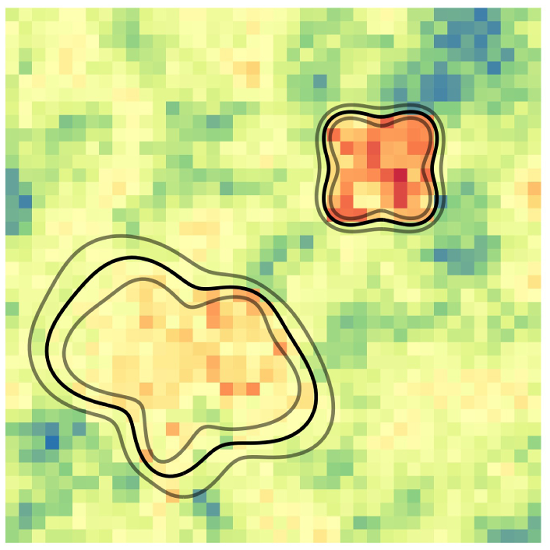
Estimated partitioning boundary (black) and 95% credible bands (grey) for one simulated dataset. Color represents voxel intensity. The procedure for simulating this data is outlined in Section 5.

5. Simulation Study

We evaluate the classification accuracy and statistical properties of BFSP-M in comparison to competing spatial partitioning and image segmentation methods through simulation. We consider a unit square image space D of 40 by 40 resolution and generate data for each region from independent Gaussian processes with Matérn covariance structures. For $j=0,1,\dots ,M$

$$\begin{gathered} {\mathit{Z}}_j\mid {\nu }_j,{\rho }_j~N\left({\mu }_j,{\Sigma }_j\right),\Sigma ={\sigma }_j^{2}H\left({\nu }_j,{\rho }_j\right)+{\tau }^2{I}_{n_j} \\ {\left(H\left({\nu }_j,{\rho }_j\right)\right)}_{i,i^{\prime }}=H\left({\nu }_j,{\rho }_j;d_{i,i^{\prime }}\right)=\frac{2^{1-{\nu }_j}}{\Gamma \left({\nu }_j\right)}{\left(\sqrt{2{\nu }_j}\frac{d_{i,i^{\prime }}}{{\rho }_j}\right)}^{\nu }{𝒦}_{{\nu }_j}\left(\sqrt{2{\nu }_j}\frac{d_{i,i^{\prime }}}{{\rho }_j}\right) \end{gathered}$$

Where $d_{i,i^{\prime }}$, is the Euclidean distance between spatial locations $s_i$ and $s_{i^{\prime }}$$,\text{Γ}$ is the gamma function, ${𝒦}_{\nu }$ is the modified Bessel function, $\nu$ is a smoothness parameter, and $\rho$ is a spatial range parameter.

To test the robustness of our method, we consider two different scenarios with either zero or two targeted regions in the space. Here we present the results for the simulations with two targeted regions. Refer to the Supplement for simulation settings and results for data containing zero target regions. In the simulated data with $m=2$ regions, we include a large heart and a small square shaped anomalous region with means ${\mu }_1=2$ and ${\mu }_2=4$, and vary the smoothness of the target region, ${\nu }_j,j>0$, and the spatial nugget parameter, ${\tau }^2$. We fix the following settings during simulation: ${\nu }_0=1,{\rho }_0=\cdots ={\rho }_M=.05,{\mu }_0=0,{\sigma }_0^2={\sigma }_1^2=\cdots ={\sigma }_M^2=1$. We randomly generate 100 spatial data sets for each of the following settings.

1. ${\nu }_1={\nu }_2=1.5,{\tau }^2=.1$

2. ${\nu }_1={\nu }_2=.5,{\tau }^2=.1$

3. ${\nu }_1={\nu }_2=1.5,{\tau }^2=.5$

4. ${\nu }_1={\nu }_2=.5,{\tau }^2=.5$

We set the maximum number of boundaries that can be proposed $M_{\text{max}}=10$ and the minimum number of boundaries to be $M_{\text{min }}=0$. We collect $50000\text{MCMC}$ samples and remove the first 20000 as burn-in samples.

The performance of BFSP-M is evaluated in terms of the frequency of correctly estimating the number of regions, and the sensitivity, specificity, and the Dice coefficient of voxel-level classification. For the settings with two anomalous regions, we compare the classification results of BFSP-M to four competing methods, two of which are basic clustering methods, K-means (KM) with 2 clusters using the function kmeans() from the R Stats package (R Core Team, 2020) and a two-stage CART method. The two-stage method involves first estimating the partitions via CART using (Ripley, 2019). This results in a tiling of the space. The second stage is to group the partitions into two clusters via KM. The cluster of tiles with the higher mean represents the target regions. We also compare to an image segmentation method BayesImageS (BIS) (Moores et al., 2020) using R-package “bayesImageS” function mcmcPotts() for which we specified neighbors via KNN with $\text{k}=8$ and 4 blocks and set the number of clusters at 2. We also ran these three competing methods with the number of clusters equal to 3 and all resulted in worse average Dice and Sensitivity scores. We further include BFSP-1 from our previous paper (Masotti et al., 2021) which assumes the presence of one and only one partitioning boundary. We initialized the MCMC chain with a large circular boundary centered at the center of the space and run for 30,000 iterations discarding the first 10,000 as burn-in samples.

In the 400 simulated data sets, using the number of boundary groups present in at least half of post burn-in simulations, our algorithm correctly identified the number of regions in $84\text{\%}$ of the cases, identified a single boundary in $9\text{\%}$ of cases, and estimated 3 boundaries in $7\text{\%}$ of cases. Estimation of the number of distinct clusters is not possible with other competing methods in which the number of clusters must be pre-specified. Figure 3 presents the distributions of the sensitivity, specificity, and Dice coefficient in detecting the target zone across the 400 simulated datasets (100 for each of the first 4 settings). Varying the parameters of the spatial processes did not have a large effect on the accuracy of BFSP-M. Figure 3 shows in contrast, the two-stage method suffers from low sensitivity and KM tends to have low specificity. BFSP-M maintains both high sensitivity and specificity in all simulation settings. Due to the large difference in means of the two target regions, BayesImages often fails to identify both regions. On average, BFSP-M achieves a sensitivity of 0.841, specificity of 0.975, and Dice coefficient of 0.842.

Figure 3:

Distributions of sensitivity, specificity, and Dice coefficient of BFSP-M, KM, Two-Stage CART, BayesImageS, and BFSP-1 over 400 simulated data sets.

The average sensitivity, specificity, and Dice coefficient are provided for each of the first 4 settings Supplementary Table 1 along with results for competing methods. Our method is robust to varying spatial smoothness. Average sensitivity is greater than $75\text{\%}$, in all scenarios, and average specificity is at least $97\text{\%}$ for all simulation settings. BFSP-M maintains average Dice coefficient of at least 0.77 over all settings.

To visualize the average classification performance we summarize the results of 100 simulations for the first setting by averaging the estimated cluster memberships based on the estimated partitions. Figure 4 presents the probability that each voxel was included in a target region for BFSP-M, KM, the two-stage CART method, BIS and BFSP-1. The BFSP-M method leads to the best contrast in color between the two target regions and the background, indicating both a high sensitivity in the target zone detection and high specificity of the outer region. The heart shaped region was more difficult to detect for all methods because its mean is relatively close to that of the outer region. The two-stage method often misses the heart shaped region altogether, explaining the low sensitivity seen in Figure 3. KM consistently identifies the target region, but does not guarantee spatial contiguity of the regions and thus random locations in the outer region are incorrectly assigned to the target region resulting in low specificity as seen in Figure 3. On average, BayesImageS identifies both regions but is more likely to missclassify voxels in the outer region than BFSP-M. BFSP-1 performs poorly due the assumption that only one target region is present in the data. BFSP-M is the only method that simultaneously estimates the number of separate regions and the voxel-wise cluster membership.

Figure 4:

From left to right: average partitioning results of the BFSP-M, KM, Two-Stage CAFT, BayesImageS, BFSP-1 methods in the simulation study. Each image represents 100 simulations of the first simulation setting. The color represents the proportion of time the method classified each spatial location as within a target region with red close to 1 and blue close to 0. The black outline shows the true boundaries.

Additional simulation results evaluating the performance of BFSP-M in the presence of zero lesions are presented in the Supplement. Our results indicate that BFSP-M was highly likely to correctly identify no anomalous regions when the covariance structure is correctly specified, but performance is somewhat degraded when the covariance is misspecified.

6. Data Analysis

We aim to validate our method as the second and final stage of a fully automated lesion detection pipeline. First we describe the dataset consisting of MRI images co-registered with the ground truth voxel-wise cancer status. Then we describe the first stage of our pipeline which is a voxel-wise prediction model developed by Jin et al. (2018). Finally, we describe how BFSP-M is applied to those outputs.

Metzger et al. (2016) present a set of data of men who received an MRI study before prostatectomy as treatment for prostate cancer. The prostates were sectioned in planes to match in vivo imaging. The sectioned prostates were digitized, allowing the pathologist to annotate and label the regions of cancer. These labeled regions were then co-registered to the imaging data to create the ground truth for disease through which the models were trained and validated. This process is detailed in Kalavagunta et al. (2015). The mpMRI data are composed of 34 prostate slices, obtained from 34 patients, with 2098 to 5756 voxels per slice.

Previously our group developed a voxel-wise prediction model for prostate cancer using the mpMRI data detailed above. The goal of this analysis is to further develop a pipeline from imaging to lesion detection using non-invasive methods. Using the results from the predictive model of Jin et al. (2018), we aim to identify the cancerous lesions within the prostate using BFSP-M. We specifically apply our partitioning method to the results of the “mregion” classifier, which models the mpMRI parameters and cancer risk by voxel coordinates and outputs a probability heatmap with values between 0 and 1.

Our aim is to translate a heatmap of cancer probabilities into one or more contiguous regions of cancer. We selected the 2 slices for which there was more than one cancerous lesion. Then we selected another 9 slices containing one lesion for which the the voxelwise classifier of Jin et al. (2018) was most successful at predicting the true voxel-wise cancer status. This allows us to focus on the performance of our segmentation relative to the ground truth, whereas an application for which the underlying voxel-wise classifier is misaligned with the ground truth will result in misaligned segmentation regardless of the performance of our method. The BFSP-M model is applied to each slice separately. We center and scale the $\left[0,1\right]$ data for each patient before applying our method. We calculate true and false positive and negative rates using the true cancer status of each voxel to measure accuracy.

We compare BFSP-M to competing spatial clustering and image segmentation methods CART, KM, BayesImageS, and our previous method BFSP-1. First we scale each slice such that all voxels fall within the unit square. We initialize BFSP-M with ${\mu }_0=0,{\mu }_1=1$, all variance parameters set to 1, and one boundary set to be a small circle centered at the voxel with the highest probability. We collect 50,000 iterations and discard the first 10,000 based on convergence of the boundary points $B$. Samples of posterior boundary coefficients corresponding to centroid groups that were not present in at least half of the MCMC samples are discarded as in Section 5. The minimum number of possible boundaries is set to be 1 because we have prior knowledge that all slices contain cancer. The maximum number of boundaries is set to be 10. We fixed the maximum number of boundaries at 10 as a conservative upper bound. The true number of lesions is less than 5 in all tested slices. Also, the MCMC sampler never visited the maximum of 10 in any of the slices. The user may consider alternate values for $M_{\text{max}}$ for other applications. For competing methods we use the same initial settings as discussed in Section 5. For BFSP-1 we use the same initial settings as BFSP-M.

Figure 5 shows the results of lesion detection for three images by BFSP-M, KM, Two-Stage CART, BayesImageS, and BFSP-1. The drawbacks of linear boundaries are clear. The estimates from CART are not reasonable for these data, which contain non-rectangular shaped regions of heightened risk. KM identifies spurious extra regions because it is not constrained to identify contiguous areas. Both methods often fail to capture the entire lesion due to their inability to account for spatial smoothness in the data. BFSP-1 will only identify one region, therefore, when multiple are present in the data as in row 1 of Figure 5, the estimated boundary covers several lesions and severly overestimates the extent of the cancer. BayesImageS and BFSP-M find spurious regions of interest but tend to identify the entire cancerous region quite well. Supplemental Table 2 presents sensitivities, specificities, and Dice scores are presented for BFSP-M and all competing methods for each of the 11 slices.

Figure 5:

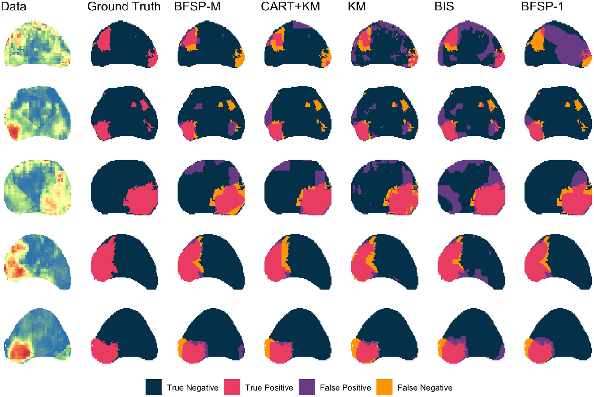
From left to right: Map of voxelwise predicted cancer probabilities from five slices where color indicates probability of cancer with red close to 1 and blue close to 0 (Jin et al., 2018), true cancer status, partitioning results from BFSP-M, Two-Stage CART, KM, BayesImageS, and BFSP-1.

Credible bands can be computed for each discovered lesion as in Section 4. See Supplementary Figure 3 for 95% credible bands for one prostate imaging slice. In addition to the boundary uncertainty, we can also compute the uncertainty of each detected lesion. Lesion uncertainty is determined by calculating the proportion of times that each centroid group appears in an MCMC posterior sample. Figure 6 displays the lesion uncertainty for two slices of data that contain multiple distinct lesions. The color of each lesion corresponds to the proportion of MCMC samples in which that lesion is present. Lesions colored red appear in all or almost all of the post burn-in MCMC samples whereas, lesions colored pale green appear less often in MCMC sampling. This result is consistent with the data which displays a high degree of noise and weak signal for several of the true cancerous lesions.

Figure 6:

From left to right: Map of voxelwise predicted cancer probabilities derived from mpMRI data from 2 slices containing multiple lesions, where color indicates probability of cancer with red close to 1 and blue close to 0 (Jin et al., 2018), true cancer status, lesion uncertainty of BFSP-M where color indicates the proportion of time that a lesion was included in the MCMC posterior draws post burn-in.

7. Discussion

We propose BFSP-M, a novel approach to accurately define spatial partitions in spatially registered imaging data containing multiple anomalous zones. BFSP-M uses functional estimation tools within multiple separate moving polar systems for boundary estimation. By allowing a minimum of zero boundaries, we can also identify data that is generated by a stationary process. We model spatial processes within each region to capture the spatial correlations present in the mpMRI data. Using novel boundary-defined jump steps in RJ-MCMC and likelihood approximations we have developed a computationally efficient method for detecting an unknown number of anomalous regions or “hot spots” in imaging data. Unlike competing methods, BFSP-M automatically detects the number of lesions, is flexible enough to detect lesions of arbitrary shape, and is able to evaluate uncertainty in boundary estimation. Further, our novel statistical framework allows for multi-subject and longitudinal analysis.

Extending the methods to accommodate the detection of an unknown number of regions adds a layer of computational complexity to our previous method, BFSP-1. First, the algorithm requires a longer burn-in period as the birth/death steps slow convergence. Furthermore, adding partitions slows computation of the posterior due to the higher dimension of the parameter space. We have implemented two key strategies to ensure BFSP-M is computationally efficient. First, we employ likelihood approximation to speed computation of the posterior. Second, we use adaptive MH sampling to encourage acceptance of proposals in MCMC. Lastly, we sample parameters in blocks to encourage mixing and decrease the number of times the likelihood must be computed. BFSP-M completed 50,000 iterations in an average time of 6.9 hours for the simulated data containing 1600 voxels.

With a birth and death process, we found that our method tended to overestimate the number of boundaries needed to partition the space into regions of local homogeneity. Without the ability to merge two boundaries, the MCMC could converge on a local maximum of the posterior where one target region is being estimated to be two separate GPs with very similar estimates of the spatial distributions. The merge step allows the MCMC to jump to a solution in which one boundary encloses both regions with one GP. With the implementation of the split and merge steps, BFSP-M estimates the true number of boundaries in 84% of datasets.

One of the advantages of the functional tools used to estimate the boundaries is that they lend themselves well to theoretical extensions. There are several avenues to further extend our methods. Our current approach limits analysis to one image slice at a time. However, a patient’s entire dataset consists of multiple imaging slices, around 10 slices per patient. A model which leverages a patient’s entire dataset may improve localization of cancer and allow estimates of cancer volume. In our framework, we could extend the spatial modeling to include correlations in the $\text{x},\text{y}$ and $\text{z}$ directions. The boundary function can be extended to be a function of two angles in the spherical coordinate system allowing estimation of boundary surfaces in three-dimensional images. This method would produce boundary surface estimates as well as 95% credible surfaces in 3D. This extension could produce highly useful visualizations to our clinical partners as they work to diagnose and assess severity for each individual patient. A multi-patient hierarchical model may also improve cancer lesion prediction by allowing characteristics about the cancer lesions to be shared among all patients. In this paper, we opted for a single patient model under the assumption that possible improvements in accuracy did not justify the computational cost. Further, our primary aim was to produce lesion estimates for each patient as their individual data became available, which is best accomplished with a single patient model. Despite this, we think a multi-patient model may be useful to explore in the future. The framework of BFSP could also be extended to model lesion boundaries over time to track disease progression. We leave this too for future study.

References

- Ahmed HU, El-Shater Bosaily A, Brown LC, Gabe R, Kaplan R, Parmar MK, Collaco-Moraes Y, Ward K, Hindley RG, Freeman A, Kirkham AP, Oldroyd R, Parker C, and Emberton M (2017). “Diagnostic accuracy of multi-parametric MRI and TRUS biopsy in prostate cancer (PROMIS): a paired validating confirmatory study.” The Lancet, 389(10071): 815–822. URL 10.1016/S0140-6736(16)32401-1 [DOI] [PubMed] [Google Scholar]
- Argiento R and De Iorio M (2022). “Is infinity that far? A Bayesian nonparametric perspective of finite mixture models.” The Annals of Statistics, 50(5). [Google Scholar]
- Banerjee S, Carlin BP, and Gelfand AE (2014). Hierarchical modeling and analysis for spatial data. Boca Raton, Florida: CRC press. [Google Scholar]
- Breiman L, Friedman J, Stone CJ, and Olshen RA (1984). Classification and regression trees. Boca Raton, Florida: Chapman & Hall/CRC. [Google Scholar]
- Chipman HA, George EI, and McCulloch RE (2002). “Bayesian Treed Models.” Machine Learning, 48(1/3): 299–320. [Google Scholar]
- Denison DG, Mallick BK, and Smith AF (1998). “A Bayesian CART algorithm.” Biometrika, 85(2): 363–377. URL https://academic.oup.com/biomet/article/85/2/363/298822 [Google Scholar]
- Denison DGT and Holmes CC (2001). “Bayesian Partitioning for Estimating Disease Risk.” Biometrics, 57(1): 143–149. [DOI] [PubMed] [Google Scholar]
- Fei B (2017). “Computer-aided diagnosis of prostate cancer with MRI.” Current opinion in biomedical engineering, 3: 20–27. URL https://pubmed.ncbi.nlm.nih.gov/29732440https://www.ncbi.nlm.nih.gov/pmc/articles/PMC5931723/ [DOI] [PMC free article] [PubMed] [Google Scholar]
- Fruhwirth-Schnatter S, Celeux G, and Robert CP (2019). Handbook of Mixture Analysis. CRC press. [Google Scholar]
- Gramacy RB and Lee HKH (2008). “Bayesian Treed Gaussian Process Models With an Application to Computer Modeling.” Journal of the American Statistical Association, 103(483): 1119–1130. [Google Scholar]
- Green PJ (1995). “Reversible jump Markov chain Monte Carlo computation and Bayesian model determination.” Biometrika, 82(4). [Google Scholar]
- Hartigan J (1990). “Partition models.” Communications in Statistics - Theory and Methods, 19(8): 2745–2756. [Google Scholar]
- Jain AK (2010). “Data clustering: 50 years beyond K-means.” Pattern Recognition Letters, 31(8): 651–666. URL 10.1016/J.PATREC.2009.09.011 [DOI] [Google Scholar]
- Jin J, Zhang L, Leng E, Metzger GJ, and Koopmeiners JS (2018). “Detection of prostate cancer with multiparametric MRI utilizing the anatomic structure of the prostate.” Statistics in Medicine, 37(22). [DOI] [PMC free article] [PubMed] [Google Scholar]
- — (2022). “Bayesian spatial models for voxel-wise prostate cancer classification using multi-parametric magnetic resonance imaging data.” Statistics in Medicine, 41(3): 483–499. [DOI] [PMC free article] [PubMed] [Google Scholar]
- Kalavagunta C, Zhou X, Schmechel SC, and Metzger GJ (2015). “Registration of in vivo prostate MRI and pseudo-whole mount histology using Local Affine Transformations guided by Internal Structures (LATIS).” Journal of magnetic resonance imaging : JMRI, 41(4): 1104–1114. [DOI] [PMC free article] [PubMed] [Google Scholar]
- Kang J, Reich BJ, and Staicu A-M (2018). “Scalar-on-image regression via the soft-thresholded Gaussian process.” Biometrika, 105(1): 165–184. [DOI] [PMC free article] [PubMed] [Google Scholar]
- Kim H-M, Mallick BK, and Holmes CC (2005). “Analyzing Nonstationary Spatial Data Using Piecewise Gaussian Processes.” Journal of the American Statistical Association, 100(470): 653–668. [Google Scholar]
- Konomi BA, Sang H, and Mallick BK (2014). “Adaptive Bayesian Nonstationary Modeling for Large Spatial Datasets Using Covariance Approximations.” Journal of Computational and Graphical Statistics, 23(3): 802–829. [Google Scholar]
- Lee CJ, Luo ZT, and Sang H (2021). “T-LoHo: A Bayesian Regularization Model for Structured Sparsity and Smoothness on Graphs.” 35th Conference on Neural Information Processing Systems. URL https://github.com/changwoo-lee/TLOHO. [Google Scholar]
- Leng E, Spilseth B, Zhang L, Jin J, Koopmeiners JS, and Metzger GJ (2018). “Development of a measure for evaluating lesion-wise performance of CAD algorithms in the context of mpMRI detection of prostate cancer.” Medical Physics, 45(5): 2076–2088. [DOI] [PMC free article] [PubMed] [Google Scholar]
- Li M and Ghosal S (2017). “Bayesian detection of image boundaries.” The Annals of Statistics, 45(5). [Google Scholar]
- Masotti M, Zhang L, Leng E, Metzger GJ, and Koopmeiners JS (2021). “A novel Bayesian functional spatial partitioning method with application to prostate cancer lesion detection using MRI.” Biometrics, n/a(n/a): 1–12. URL https://onlinelibrary.wiley.com/doi/abs/10.1111/biom.13602 [DOI] [PMC free article] [PubMed] [Google Scholar]
- Metzger GJ, Kalavagunta C, Spilseth B, Bolan PJ, Li X, Hutter D, Nam JW, Johnson AD, Henriksen JC, Moench L, Konety B, Warlick CA, Schmechel SC, and Koopmeiners JS (2016). “Detection of Prostate Cancer: Quantitative Multiparametric MR Imaging Models Developed Using Registered Correlative Histopathology.” Radiology, 279(3): 805–816. [DOI] [PMC free article] [PubMed] [Google Scholar]
- Moores M, Nicholls G, Pettitt A, and Mengersen K (2020). “Scalable Bayesian Inference for the Inverse Temperature of a Hidden Potts Model.” Bayesian Analysis, 15(1). [Google Scholar]
- Neal RM (2000). “Markov Chain Sampling Methods for Dirichlet Process Mixture Models.” Journal of Computational and Graphical Statistics, 9(2): 249–265. URL http://www.jstor.org/about/terms.html. [Google Scholar]
- Page GL and Quintana FA (2016). “Spatial Product Partition Models.” Bayesian Analysis, 11(1). [Google Scholar]
- R Core Team (2020). “R: A Language and Environment for Statistical Computing.”
- Richardson S and Green PJ (1997). “On bayesian analysis of mixtures with an unknown number of components.” Journal of the Royal Statistical Society. Series B: Statistical Methodology, 59(4): 731–792. [Google Scholar]
- Ripley B (2019). “tree: Classification and Regression Trees.”
- Roberts GO and Rosenthal JS (2009). “Examples of Adaptive MCMC.” Journal of Computational and Graphical Statistics, 18(2): 349–367. [Google Scholar]
- Salvador S and Chan P (2004). “Determining the number of clusters/segments in hierarchical clustering/segmentation algorithms.” In 16th IEEE International Conference on Tools with Artificial Intelligence, 576–584. [Google Scholar]
- Sugar CA and James GM (2003). “Finding the Number of Clusters in a Dataset: An Information-Theoretic Approach.” Journal of the American Statistical Association, 98(463): 750–763. [Google Scholar]
- Teixeira LV, Assunção RM, and Loschi RH (2019). “Bayesian Space-Time Partitioning by Sampling and Pruning Spanning Trees.” Journal of Machine Learning Research, 20: 1–35. URL http://jmlr.org/papers/v20/16-615.html. [Google Scholar]
- Wendland H (1995). “Piecewise polynomial, positive definite and compactly supported radial functions of minimal degree.” Advances in Computational Mathematics, 4: 389– 396. [Google Scholar]
Associated Data
This section collects any data citations, data availability statements, or supplementary materials included in this article.