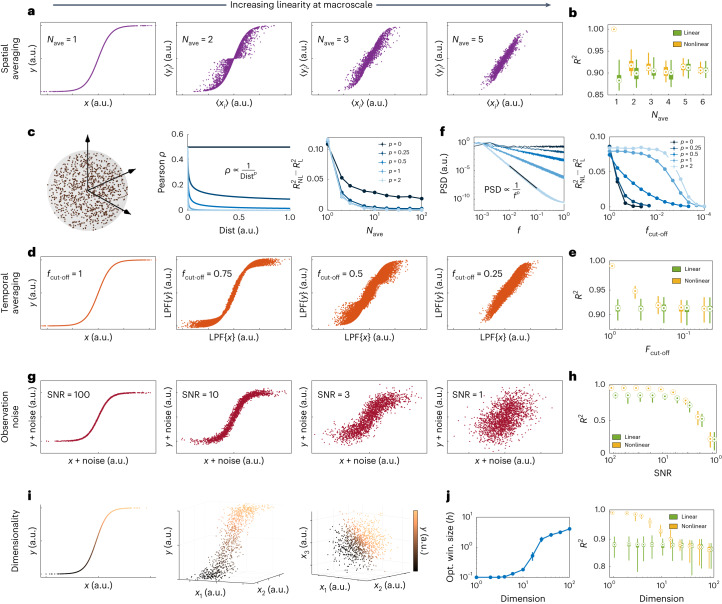
Fig. 4. The linearizing properties of macroscopic brain dynamics and of neuroimaging measurements.
a, The effect of spatial averaging. For each panel, Nave pairs of signals xi(t), t = 1,…,2,000 were randomly and independently generated, was calculated, and their averages 〈xi〉 and 〈yi〉 were computed. The quantities 〈xi〉 and 〈yi〉 possess a linear relationship as Nave ≈ 5 or higher. b, The cross-validated R2 of the optimal nonlinear (MMSE) and linear predictors for the 〈xi〉–〈yi〉 relationships in a. c, The effect of spatial correlation on spatial averaging. Here we assign (xi(t),yi(t)) pairs to spatial locations in a unit sphere (left) and make each xi(t) and xj(t) correlated in a manner that depends on their spatial distance (middle). The difference between nonlinear and linear R2 always decays with Nave and vanishes if the correlation decays, even slowly, with distance (right). d, The effect of temporal averaging. One pair of was generated, independently over time and passed through a Gaussian low-pass filter (LPF) with a cut-off frequency fcut-off that is normalized to the Nyquist frequency; thus, fcut-off = 1 means no LPF. e, Same as b but for the LPF{x}–LPF{y} relationships in d. f, Similar to c but for temporal averaging. We varied the PSD decay rate of x(t) (left) and then low-pass filtered x(t) and as in d. The difference between the optimal linear and nonlinear R2 eventually vanishes as fcut-off decreases, but it happens at smaller fcut-off for larger decay rates p (right). g, The effect of observation SNR. The quantities x(t) and and y(t) = tanh(x(t)) are as in d and their additive noises were generated independently. h, Same as e but for the (x + noise) − (y + noise) relationships shown in g. i, The effect of dimensionality. The values x1(t),…,xn(t) were generated as in a but here y(t) = tanh(x1(t)…+xn(t)) generates a one-dimensional nonlinearity in n + 1 dimensions. No noise is included; no spatial or temporal averaging is applied. j, Right: similar to b, e and h except that a manifold-based (locally linear) nonlinear predictor was used since the conditional density estimation required for MMSE loses accuracy in high dimensions with a fixed number of data points (see Methods). Left: the optimal window size of the manifold-based predictor as a function of dimension n. As n increases, the locally linear predictor automatically chooses larger windows to be able to make reliable predictions, thereby effectively degrading to a globally linear predictor (see also Supplementary Fig. 1). In all boxplots, the centre point, box limits and whiskers represent the median, upper and lower quartiles, and the smallest and largest samples, respectively. Error bars in c, f and j represent 1 s.e.m.

