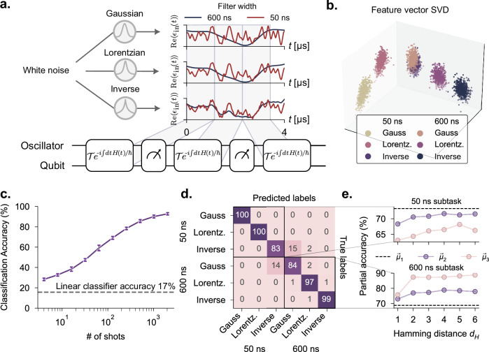
Fig. 4. Classification of filtered noise.

a We classify various fast and slow noisy signals by applying a moving average on stochastic white-noise signals. Three different filters are used for the moving averages: a Gaussian filter, a Lorentzian, and an inverse power law. For each filter, we generate stochastic analog signals based on both a 50 ns filter width, and a 600 ns filter width, with the latter being on the order of the measurement rate. Example time traces are given for the real part of an example stochastic white noise signal passed through each of the filters. We divide up these stochastic signals and send to the QRC to then distinguish the noise source. b Visualization of the high-dimensional output feature space using Singular Value Decomposition (SVD). Each point corresponds to a different signal over 2000 shots taken in real time (see text). c Classification accuracy as a function of the number of shots using third-order moments as the output feature. Our reservoir reaches 93% accuracy in about 2000 shots, corresponding to about 10 ms of the signal received. The errorbars here indicate the variation in the classification accuracy over the testing dataset. d Confusion matrix of the task taken at 2000 shots. e Participation of the mean and the off-diagonal elements of the second- and third-order moments in the classification accuracy within the subtasks of classifying different noise sources with fixed filter width. We see that for signals with long coherence times, higher-order measurement correlations are important, while for fast signals, the mean dominates in the performance contribution.