FIGURE 5.

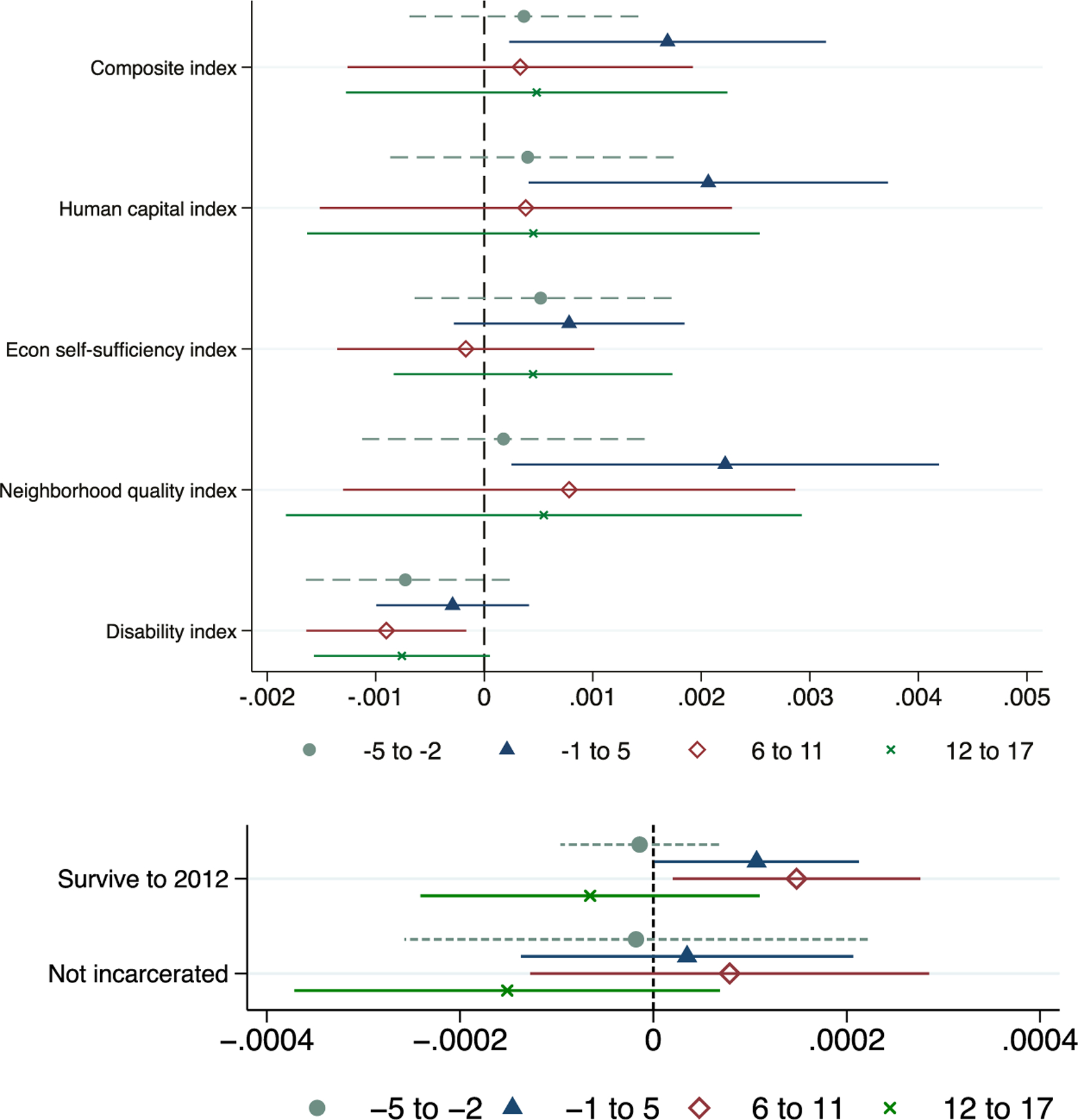
ITT spline estimates of effects of Food Stamps, by age of cohort when the program launched

Notes: These figures plot the absolute values of the estimates (and their associated 95% confidence intervals) on the four linear spline segments in equation (2) for each outcome listed along the y-axis. In particular, we plot $\text{—}{\omega }_1\text{—}$ (ages −5 to −2), $\text{—}{\omega }_2\text{—}$ (ages −1 to 5), $\text{—}{\omega }_3\text{—}$ (ages 6–11), and $\text{—}{\omega }_4\text{—}$ (ages 12–17), where age is when Food Stamps launched in their county of birth. The sample includes more than 17 million U.S. individuals born in the U.S. between 1950 and 1980 who are observed in the 2000 Census one-in-six sample and 2001–13 ACS merged to the SSA’s NUMIDENT file using PIKs. The regressions are estimated on data collapsed into birth-county × birth-year × survey-year cells, and weighted using the number of observations per cell. Standard errors clustered at the birth-county level. See text for more information on the construction of the sample and the outcomes. Note that the indices are standardized in terms of standard deviations, but “survive to 2012” and “not incarcerated” are not, which is why these latter two outcomes appear on different scales. All models include fixed effects for birth county, birth state × birth year, and survey year, as well as 1960 county characteristics interacted with a linear trend in year of birth.