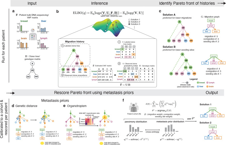
Figure 1. Overview of the Metient method.

(a) Input: (top) bulk DNA sequencing sampled from multiple tumors in a single patient, and (bottom) a clone tree which represents the evolutionary relationship of mutations. AB refers to a clone with mutations or mutation clusters A and B. (b) Inference: Using the inputs as observed variables, we infer the latent variables (1) $\mathbf{V}$ (representing the labeled clone tree) and (2) $\mathbf{U}$ (representing the proportion of each clone in each anatomical site). $\stackrel{\mathbf{ˆ}}{\mathbf{F}}$ is the estimated VAF matrix produced by $\mathbf{U}\mathbf{B}$, where ${\mathbf{B}}_{ij}=1$ if clone $i$ contains mutation $j$. Each migration history solution can be represented by a migration history, which is a clone tree with (1) an anatomical site labeling of its internal nodes, and (2) leaf nodes representing the observed clone proportions in anatomical sites. (c) Identify Pareto front of histories: We infer a Pareto front of migration histories as defined by the three parsimony metrics (migration, comigration and seeding site number). A migration graph $\mathbf{G}$ summarizes the migration edges of the migration history. (d) Genetic distance: An example of how using genetic distance can promote migration histories with migrations on longer edges with more mutations. The anatomical site label of the yellow shaded node is changed. (e) Organotropism: An example of how using organotropism can promote migration histories that do not contain unlikely metastatic patterns, such as subsequent metastasis from the brain. The anatomical site label of the yellow shaded node is changed. (f) Metient-calibrate: Weights on the parsimony metrics ($\theta$) are fit by minimizing the cross entropy loss between each patient’s migration histories’ probability distribution as scored by the metastasis priors (target distribution) and the probability distribution as scored by the parsimony metrics (source distribution). These weights are fit across a cohort of patients, and then used to rescore the Pareto front of migration histories produced for each patient in that cohort.