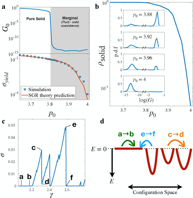
FIG. 1.

(a) Discrepancy between shear start-up and steady-shear regime. Top: The shear modulus of the un-sheared tissue $(\mathrm{\gamma }=0)$. The shear modulus is obtained using linear-response calculation (see Methods). Bottom: The yield stress ${\mathrm{\sigma }}_{yield}$ obtained from the steady-state shear regime of quasistatic simulations is shown together with the yield stress obtained from the SGR model, where the only fitting parameter in the model, the elastic constant of an element was chosen to be $k=0.0386$. (b) The probability of finding the system in solid state as a function of $p_0$. Inset: Distribution of tissue stress at different $p_0$. (c) Stress-strain curve example showing different yielding types: a fluid state yields to another fluid states $\mathbf{a}\to \mathbf{b}$, a solid state yields to another solid one $\mathbf{c}\to \mathbf{d}$, and a solid state yields to a fluid state $\mathbf{e}\to \mathbf{f}$. (d) Schematic of the dynamics of elements in the SGR model: The energy landscape of the material consists of traps with different depth $E$ drawn from a distribution $\mathrm{\rho }(E)$ that characterizes the structural disorder of the material. Yielding events are captured by transitions from one trap to another. The three types of transition illustrates the transitions observed in simulation