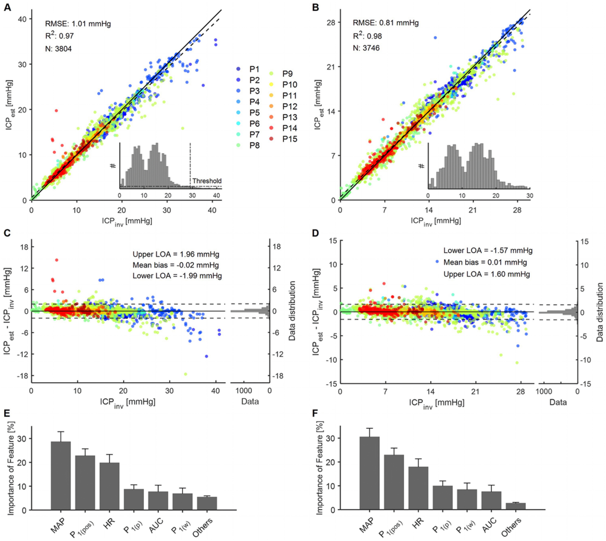
FIG. 4.

Results of the regression forest machine learning model for the entire range of ICPinv (0.01–41.25 mm Hg) and a narrower range of ICPinv (0.01–29.05 mm Hg). The data points are color coded according to patient identification. A–B: Performance of the regression forest. The solid line shows the ideal fit between ICPinv and ICPest, whereas the dashed line shows the linear fit. R2 represents goodness of fit, and N represents the sample size of the testing set. The inset images show histograms of ICPinv of the entire sample population before splitting into the train/test sets. A bin width of 0.83 mm Hg was used in the histogram. C–D: The Bland-Altman plot shows the difference between the two methods with respect to ICPinv. The solid line represents mean bias and the dashed lines represent the upper and lower 95% LOA. The histogram plots on the right side of each panel display the distributions of the differences. E–F: Distribution of features used in the regression forest model as a percentage of all chosen features of all decision criteria generated. The standard deviation across 200 individual trees is shown as error bars. Others refers to all other features apart from the ones shown in the plot. For nomenclature, please see the Signal Processing section of the Methods and Fig. 2C. LOA = limit of agreement.
