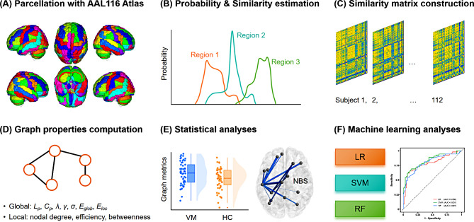
Fig. 1.

Flowchart of the analysis process. (A) The GM volume was estimated with VBM using SPM. Whole-brain GM was parcellated using the AAL116 atlas (116 regions). (B) The PDF of GM volume was calculated using kernel density estimation. Statistical similarities between the PDFs of pairwise brain regions were then evaluated with KL divergence. (C) As a result, a 116 × 116 similarity matrix representing the GM volume covariance network was generated for each subject. (D) Global and local topological properties were calculated through graph-theoretical analyses. (E) The network metrics, including network topological properties and connections were compared between patients with VM and HCs. (F) LR, SVM, and RF classifiers were used to construct models for distinguishing individuals with VM from HCs based on the discriminative GM connectome features. GM = gray matter; VBM = voxel-based morphometry; SPM = Statistical Parametric Mapping; AAL = Automatic Anatomical Labeling; PDF = Probability Distribution Function; KL = Kullback–Leibler; VM = vestibular migraine; HC = healthy control; LR = logistic regression; SVM = support vector machine; RF = random forest; L_p = characteristic path length; C_p = clustering coefficient; λ = normalized characteristic path length; γ = normalized clustering coefficient; σ = small-worldness; E_glob = global efficiency; E_loc = local efficiency; NBS = network-based statistics; AUC = area under the curve