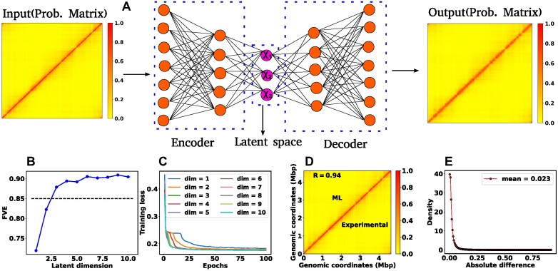
Figure 1.
Architecture of the Autoencoder and training robustness. (A) Schematic of the Autoencoder, an unsupervised machine learning algorithm. It consists of an encoder and a decoder and in between there is a bottleneck. The encoder transforms high-dimensional input data to a lower-dimensional latent space, while the decoder reconstructs the initial input data from the latent space. This process involves adjusting model parameters, primarily weights, and biases. Each dimension in the latent space corresponds to a latent variable. Here, χ1, χ2 and χ3 represent three latent variables. (B) The variation of FVE with respect to the latent dimension (Ld). A Ld = 3 was chosen, ensuring an FVE of at least 0.85, signifying that the Autoencoder’s reconstruction captures a minimum of  of the variance in the input data. (C) Training loss as a function of epochs for different latent space dimensions (Ld). Notably, the training loss achieves saturation for all Ld > 1 beyond 25 epochs. (D) Genome-wide contact probability map between the experimental and ML-derived Hi-C matrix. (E) Histogram of the absolute difference between experimental and ML-derived contact probability matrices. The Pearson correlation coefficient(PCC) is 0.94, and the absolute difference in mean values is 0.023, indicating a substantial agreement in chromosomal interactions.

