Fig. 5:

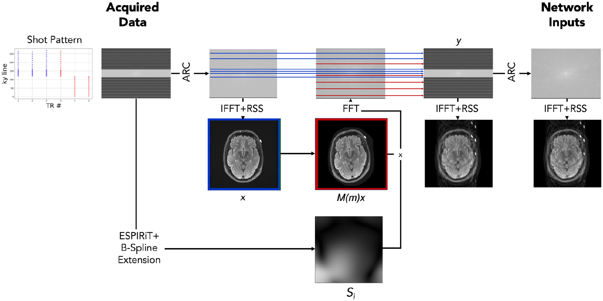
Motion simulation schematic. We apply ARC reconstruction (Brau et al., 2008) to motion-free data followed by the inverse Fourier transform and root-sum-of-squares coil combination, yielding the initial motion-free image $x$. We also estimate coil sensitivity profiles $S_i$ from the acquired data using ESPIRiT (Uecker et al., 2014) with learned parameter estimation (Iyer et al., 2020) and extend the profiles to the image edge via B-spline interpolation. Next, we simulate an image under a sampled random motion $M\left(m\right)$ by applying rotations and translations to the image and use the sensitivity maps and a Fourier transform to simulate k-space data corresponding to the moved position. Based on the shot pattern for the acquisition, we combine k-space data from the appropriate lines corresponding to the position pre- (blue) and post-motion (red) to form simulated, motion-corrupted k-space measurements $y$. This simulates the k-space data that would have been acquired had the subject moved from the blue position to the red position over the course of the acquisition. The input to our networks is the ARC reconstruction of this simulated $y$. In practice, we sample two versions of $M\left(m\right)x$ and treat one of the two as $x$, to avoid discrepancies between simulated and acquired data when mixing the k-space.