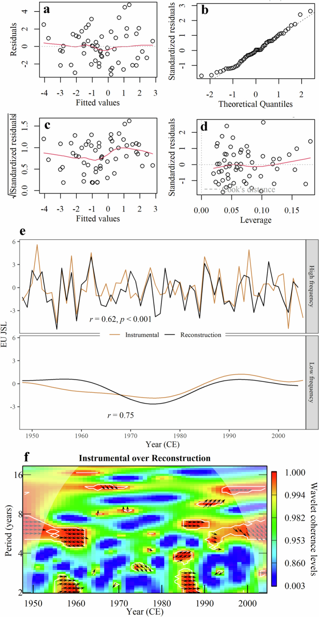
Extended Data Fig. 4. Variability and distribution of the residuals derived from the multiple linear regression reconstruction model and comparison between reconstructed and instrumental summer EU JSL for the period 1948–2004 ce.
(a) Scatter plot between residuals and fitted values in the linear regression, (b) Q-Q plot of the standardized residuals, (c) scatter plot between standardized residuals and fitted values, and (d) scatter plot between standardized residuals and leverage values. The vertical dashed line indicates the Cook’s distance in panel (d). The comparison is shown for both high- and low-frequency variability, after applying a 20-year smoothing spline. In panel (e), r represents the Pearson correlation coefficient between reconstructed and instrumental EU JSL. For the low-frequency series, the level of significance is not provided since the effective degrees of freedom were not adjusted. Panel (f) shows a complementary cross-wavelet coherency analysis between instrumental and reconstructed summer EU JSL. Instrumental data is derived from the NCEP/NCAR reanalysis product.

