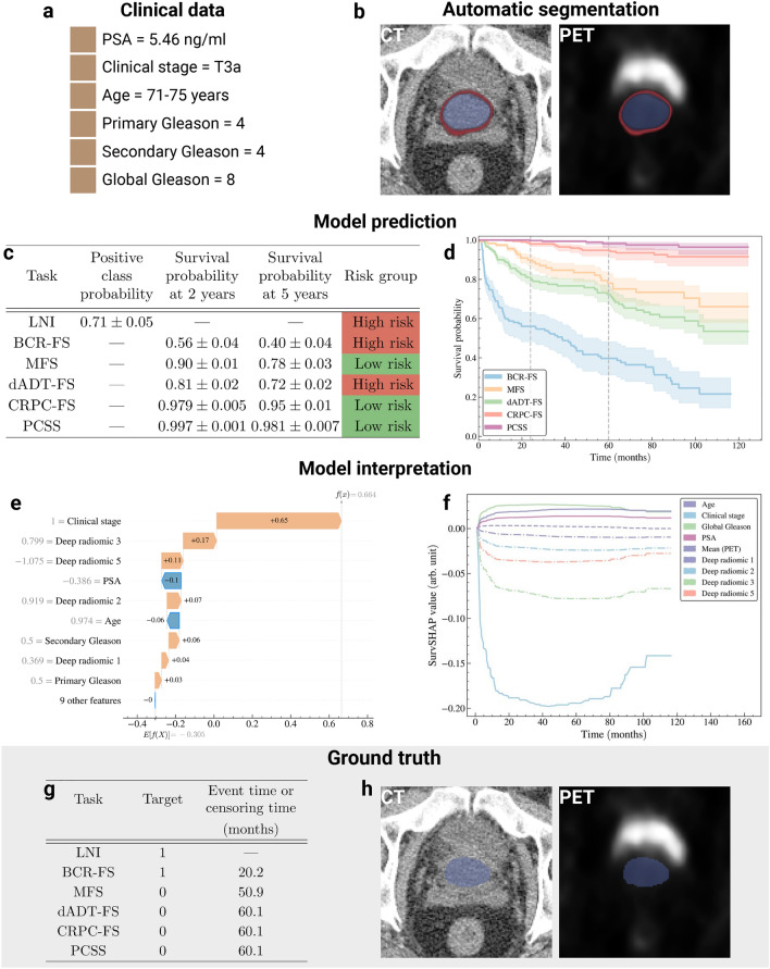
Fig. 6.

Illustration of a clinical application of selected models. The application involves establishing the prognosis of an arbitrarily selected patient from the holdout set. See Supplementary Figs. 20 & 21 for other examples of patient prognosis. (a) Patient’s clinical data. (b) Segmentation map of the prostate obtained from Bayesian U-Net trained on the learning set. The segmentation map is overlaid on CT and PET images to illustrate that the region of high FDG uptake by the bladder lies outside the segmentation map’s boundaries. The segmentation map is used to extract handcrafted radiomic features. Note that the DSC between automatic and manual segmentation (ground truth) is 0.910. Color code: average prostate segmentation map (blue) and standard deviation (red) over 100 inferences. See Supplementary Fig. 22a for the segmentation map obtained by Bayesian U-NEXtractor. (c) Average prediction and standard deviation of the model over 100 inferences. (d) Average survival curves predicted by the model (line) and 95% confidence interval (shade) over 100 inferences (e) Shapley additive explanation (SHAP)⁵⁹ of the predicted risk of BCR-FS. (f) Time-dependent SHAP (SurvSHAP(t))⁶⁰ of the predicted risk of BCR-FS. (g) Ground truth progression of the patient’s cancer. Time represents the survival time when the target value is 1 and acts as a censoring time otherwise. (h) Ground truth prostate segmentation map obtained from manual contouring by a physician. Created in BioRender. Larose, M. (2024) https://BioRender.com/r08k904.