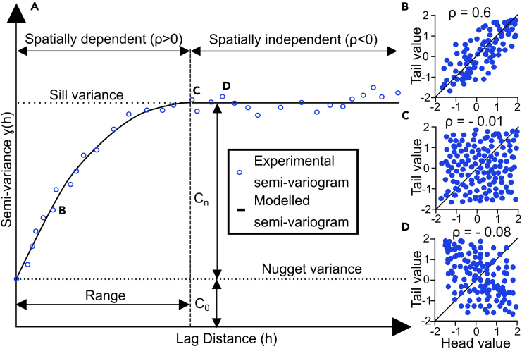
Figure 1.
Anatomy of an experimental and modelled semi-variogram
(A) Anatomy of a semi-variogram (adapted from37,41). An experimental semi-variogram is calculated through comparison of all point pairs in a particular direction for each lag (h) distance following Equation 1. Each point in the experimental variogram corresponds to the correlation coefficient (ρ) of the scatterplot along the x = y bisectrix between head and tail values of the vector between each point pair: for instance, points B, C, and D correspond to h-scatterplots (B), (C) and (D), respectively. The semi-variogram is a model of the semi-variance as a function of separation (lag, h) distance. The nugget corresponds to the semi-variance at the shortest measured separation distance. The sill variance corresponds to the maximum variance of the system. The sill allows the interpretation of the range. The range is the maximum separation distance until which there is correlation between data points (ρ < 0) and is interpreted as the separation distance at which the semi-variogram reaches the sill variance. C0 is the contribution of the nugget variance toward the total (sill) variance. Cn is the subsequent contributions of the n models necessary to model the experimental variogram. n is 1 if only one model is necessary to accurately model the system but can be 2 or more making it a nested model. See Figure 6 for an example of a nested model.

