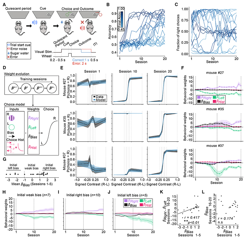
Figure 1. Idiosyncratic and side-specific learning trajectories.

(A) Schematic of the task. On each trial, a Gabor patch of a different contrast (6.12%, 12.5%, 25%, or 100%) is presented on the right or left side of a screen. Centering the patch with a steering wheel leads to a small water reward, whereas moving it out of the screen results in a short timeout (2 s) and white noise (0.5 s).

(B) Accuracy (fraction of trials rewarded) across training sessions.

(C) Probability of right choices across training sessions. In (B) and (C), each line represents one mouse, colored by their mean accuracy in sessions 16–20.

(D) Schematic of the behavioral model. Choice (left or right) on each trial is predicted with a logistic function based on weighting the contrast of the right and left visual stimulus (β_right and β_left), a bias term (β_bias) coded such that positive values indicate rightward choice, and a choice history kernel. Weights evolved across sessions (see STAR Methods for details).

(E) Psychometric curves (“data”) and model fits (“model”) from 3 example mice on the first, middle, and last session of training. Lines and shading represent mean ± SEM.

(F) Model weights across training for the same mice from (E). Lines and shading represent mean and 95% confidence intervals.

(G) Early β_bias (average of sessions 1–5) for all the mice, showing the subdivisions used in subsequent panels between mice with weak, left, or right initial bias.

(H–J) Average trajectories of bias, right and left stimulus weights across training for mice subdivided by their initial bias as shown in (G). Lines and shading represent mean ± SEM across mice.

(K and L) Relationship between early β_bias (average of sessions 1–5) and the late difference in stimulus sensitivity weights (β_right - β_left for sessions 16–20). r = 0.417, p = 0.0007.

(I) Relationship between early β_bias (sessions 1–5) and late β_bias (sessions 16–20). R = 0.174, p = 0.522.

In (K) and (L), each dot is a mouse. Correlation and p values from robust regression. **p < 0.01; ns, not significant.

Across all panels, n = 22 mice.

See also Figure S1.