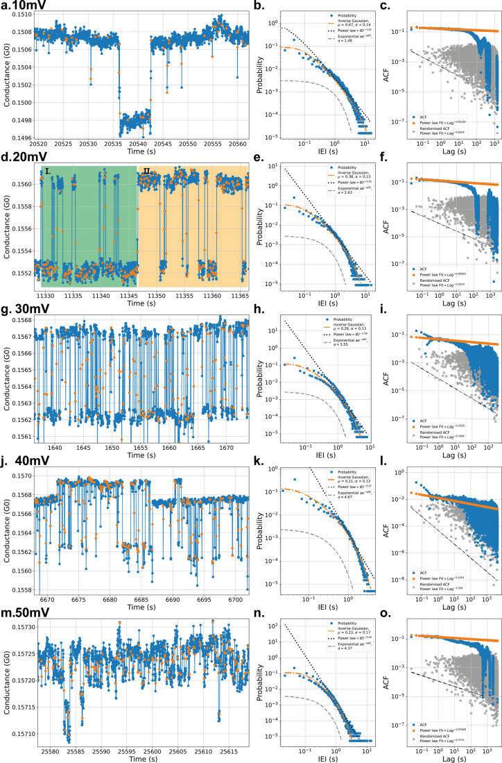
Figure 2.

Five 12-h continuous measurements of the same NP network at 10 (a.), 20 (d.), 30 (g.), 40 (j.), and 50 (m.) mV biases have been performed with respective zoomed-in sections of approximately 35 s shown in the first column. The switches have been marked in orange. Note the increase in switching frequency upon increasing the bias application. In d., levels are sometimes predominantly occupied with switching occurring rapidly toward the other level highlighted in sections I. and II. This occurs in all bias applications. In the second column (b., e., h., k., and n.), the respective (heavily tailed) PDF distributions of the IEIs are shown, with binning equal to the measurement interval. A comparison is made between three different fitting models: an inverse Gaussian fit in an orange dash-dot line; a power law fit in a black dotted line; and an exponential fit in a gray dashed line. Finally, in the last column (c., f., i., l., and o.), the respective autocorrelation functions (ACFs) are shown. In blue, the ACFs with its orange power law fit are shown. Upon shuffling the IEI sequence, correlations are lost, as seen in the gray ACF with its accompanying, black-dotted power law fit. Note: all fits are within a 95% confidence interval. The identification thresholds are 8, 5, 7.5, 5, and 2 × 10^–5 for the data sets of 10–50 mV, respectively.