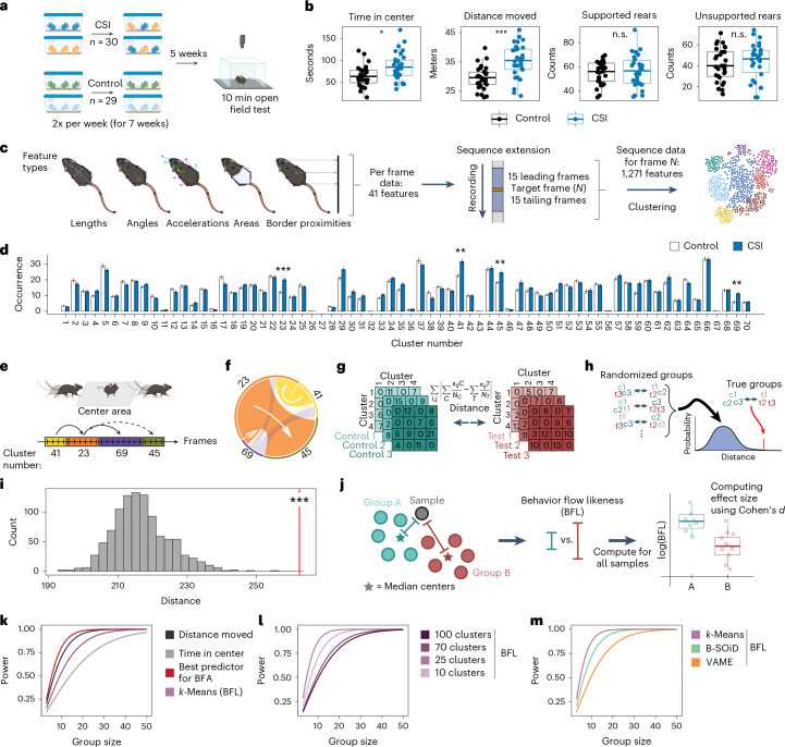
Fig. 1. BFA increases power to detect phenotypes.
a, A schematic showing the experimental design for CSI. b, Classical behavior readouts in the OFT show that CSI mice (n = 30) spend more time in the center (two-tailed t-test, t(53) = 2.96, adjusted P = 4.47 × 10⁻²) and travel greater distance (two-tailed t-test, t(52) = 4.55, adjusted P = 7.08 × 10⁻⁴) than controls (n = 29). c, Feature extraction based on pose-estimation tracking and sequential feature integration for subsequent clustering. d, The k-means cluster occurrence in CSI (n = 30, controls: n = 29; two-tailed t-tests with multiple testing correction). e, A schematic example of behavioral flow based on cluster transitions. f, The average behavioral flow over all animals between example clusters. The white arrows display the direction of transition. g, Schematic of computing Manhattan distance to compare behavioral transition matrices between groups. h, The permutation approach used for BFA to compare the transition distance based on the true group assignment versus the randomized group assignment. c, control; t, test. i, BFA reveals a treatment effect for CSI (one-tailed z-test, percentile 99.9, z = 5.72, P = 5.28 × 10⁻⁹, d = 0.97). j, Schematic of computing the BFL score to estimate effect sizes. k, Power analysis comparing classical readouts (‘distance moved’ and ‘time in center’) with analysis of cluster transitions. l, The number of clusters influences power to detect treatment effects. m, Power analysis comparing three different clustering algorithms. P values and adjusted P values are denoted as *<0.05, **<0.01 and ***<0.001; n.s., not significant. For box plots, the center line denotes the median value, while the bounding box delineates the 25th to 75th percentiles. The whiskers represent 1.5 times the interquartile range from the lower and upper bounds of the box. The error bars in the bar plot denote mean ± s.e.m.

