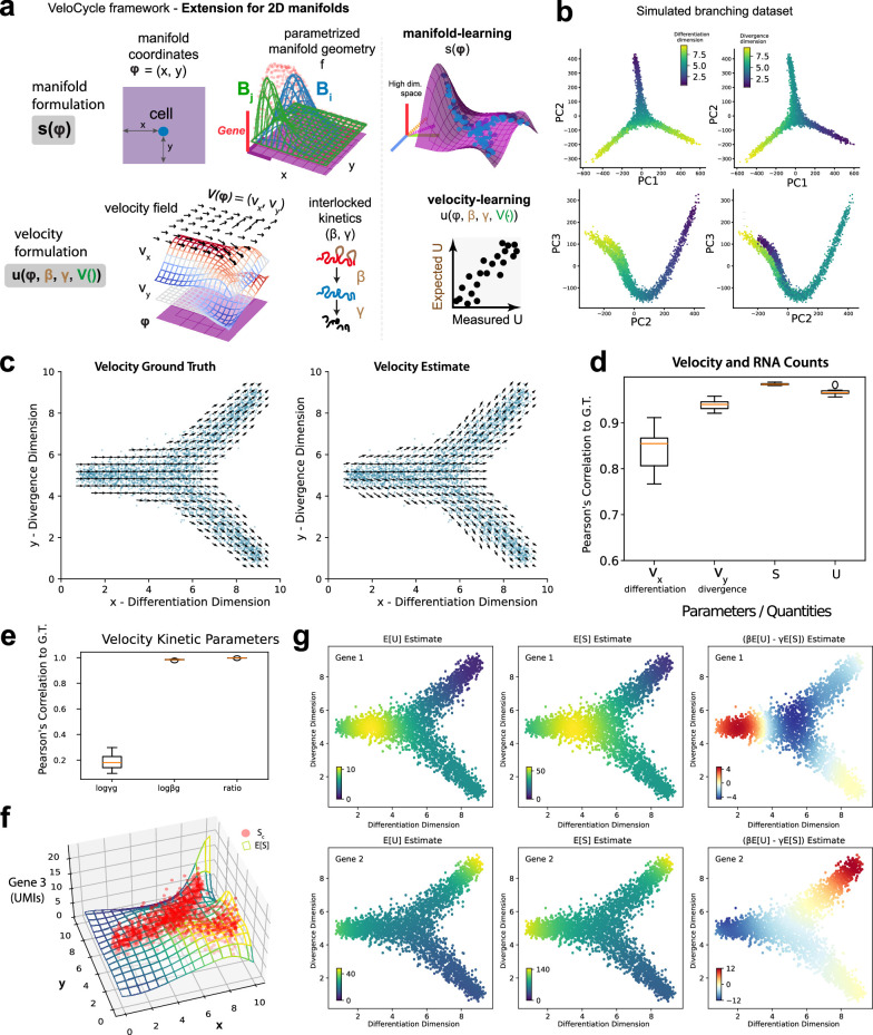
Extended Data Fig. 10. Formulation of manifold-constrained velocity analysis along a 2D axis.

(a) Schematic of the 2D manifold model, where variation in gene expression along two dimensions (defined, for example, by two principal components) is estimated using B-splines instead of a Fourier series (as in VeloCycle). (b) Simulated 2D branching dataset with estimated and ground truth (GT) velocity. Cell positions from one of the ten simulated datasets are shown in blue. Velocity and spliced mRNA counts were parameterized as 2D B-splines conditioned on the coordinates of the cells; GT velocity spline coefficients were set manually. (c) Box plots of Pearson’s correlation coefficients between the estimated and GT velocities and mean un/spliced counts. Velocities were evaluated separately along two dimensions, one corresponding to the overall differentiation process and one representing the divergence of the branches. (d) Box plots of Pearson’s correlation coefficients between the estimated and GT kinetic parameters across ten simulated datasets. Boundaries in (d) and (e) are defined by the interquartile range (IQR); whiskers extend each box by 1.5x the IQR. (e) Estimated expected un/spliced counts of two selected genes and the estimated spliced counts derivative. (f) Scatter and surface plot representing an example of a gene fit as a function of manifold location using splines. Red dots are simulated data and the mesh surface is the expectation that was fit by the manifold learning step. (g) Scatter-plots of representative genes colored by the expected S and U obtained by manifold learning and velocity learning steps. Plots on the right make the un/spliced delay easier to appreciate by coloring the scatter by a proxy for gene-wise velocity βE[U] - γE[S].