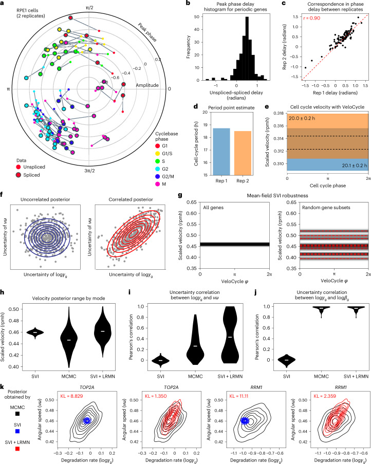
Fig. 4. Analysis of delays, velocity scale, and parameter uncertainties in the choice of variational distribution.
a, Polar plot of peak unspliced–spliced expression for 106 marker genes across two replicates of RPE1 cells analyzed with manifold learning. Genes are colored by their categorical annotation in Cyclebase 3.0 (ref. 38). Unspliced gene fits were inferred separately, conditioned on cell phases obtained when running manifold learning on spliced UMIs. b, Histogram of unspliced–spliced delays (in radians). c, Scatterplot of unspliced–spliced delays (r = 0.90) between replicates from a. d, Bar plot of cell cycle periods obtained with a first-order-approximate point estimate (Methods). e, Posterior estimate plot of constant, scaled cell cycle speed (rpmh) for the two replicates. Black dashed lines indicate a mean of 500 posterior predictions and the colored bar indicates the credibility interval (5th to 95th percentile). f, Schematic of the hypothetical scenarios where a gene has uncorrelated (left) and correlated (right) posterior uncertainty between logγg and νω. Blue circles represent the Gaussian kernel distribution density; red lines represent an uncertainty interval between two arbitrary fixed points. g, Posterior estimated velocity plot inferred for cultured human fibroblasts32 using the original SVI mode of VeloCycle and either all genes (left) or random gene subsets (50% of total genes; right). h, Violin plots of scaled velocity (in rpmh) after estimation using SVI, MCMC and LRMV (SVI + LRMN) velocity learning models. i, Violin plots of Pearson’s correlations between the degradation rate (logγg) and angular speed (νω) posterior uncertainties across 160 genes. j, Violin plots of Pearson’s correlations between degradation (logγg) and splicing (logβg) uncertainties. k, Density representation of overlapping logγg−νω posterior distributions between MCMC and either SVI (top) or SVI + LRMN (bottom) for TOP2A and RRM2 (black, MCMC; blue, SVI; red, SVI + LRMN). Kullback–Leibler (KL) divergence scores are in red. Violin plots in h–j are built from 500 predictive samples; the white line indicates the mean.

