Fig. 4.

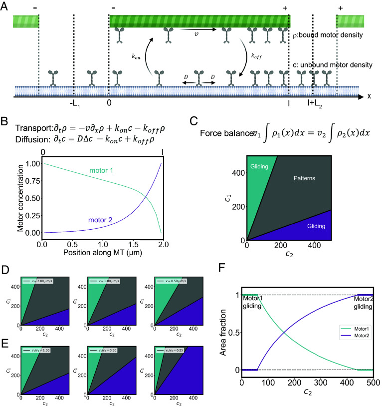
Model and simulations of microtubules and motors self-organization. (A) Schematic representation of the model parameters. In a box of length L (equal to L1 + l + L2), motors beneath a microtubule of length l are separated in two populations: bound ρ and unbound c, motors have a diffusion coefficient D, a gliding speed on the microtubule v and transition rates between the two populations kon and koff. (B) Motors diffusion and sorting along the microtubule. Top: transport and diffusion equations. Bottom: plot of the theoretical prediction of the motor concentrations profiles along the microtubule with D = 1.5 µm²/s, l = 2 µm, kon = 1 s⁻¹ koff = 25 s⁻¹ v = 0.3 µm/s for motor 1 and kon = 12 s⁻¹ koff = 1 s⁻¹ v = 0.5 µm/s for motor 2. (C) Conditions for the emergence of self-patterning. Top: force balance equation between motor 1 and motor 2. Bottom: phase diagram showing the emergence of the different behaviors in response to combinations of motor concentrations. The model predicts that the boundaries between the “gliding” and “self-patterning” behaviors in this diagram are linear (SI Appendix). (D) Phase diagrams for different gliding speeds (here v1 = v2 = v). (E) Phase diagrams for different speed ratios between the motors. (F) Size of motor domains in self-patterning conditions. The graph shows the theoretical area fraction of each motor for a given concentration of motor 1 and increasing concentration of motor 2.