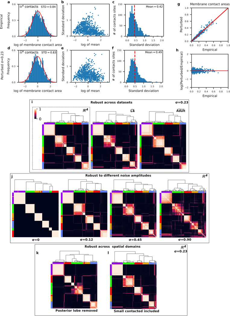
Extended Data Fig. 5. Robust clustering of nerve ring processes from ${\mathbb{M}}^4$ spatial population models.

The variability of membrane contacts (Fig. 2, Extended Data Fig. 2) suggest that no single animal is representative of the population. We estimated the variability among membrane contact areas. a, The log-normalized empirical distribution of ${\mathbb{M}}^4$ membrane contact areas (mean centered at 0, STD: standard deviation, red line: normal distribution with empirical mean and standard deviation, $n=1,258$ membrane contacts). We estimated the variability across the four datasets (L4 left, L4 right, adult left and adult right). For each conserved ${\mathbb{M}}^4$ contact, we computed the mean and standard deviation of the membrane contact area across the four datasets (see Methods). b, Plot of the standard deviation versus mean contact area across the datasets, where each point is one ${\mathbb{M}}^4$ contact. Similar to Extended Data Fig. 1a, we find no dependence of the variability on membrane contact area. Therefore, we estimate membrane contact area variability by the mean variability among all membrane contact areas. c, The distribution of standard deviations of membrane contact area for all ${\mathbb{M}}^4$ contacts. Red dashed line: mean standard deviation. d-i, A stochastic spatial population model matches the above distributions by randomly perturbing membrane contact areas in the four datasets with multiplicative white noise with standard deviation ($\sigma$) of 0.23 (Methods). d-f, Spatial population data perturbs the membrane contact areas while maintaining contact area and variability distributions that are similar to the empirical ${\mathbb{M}}^4$ contact area distributions. g, Perturbed contact areas scale linearly with the empirical contact areas. h, The spread of perturbed contact areas (log of the perturbed contact area as a fraction of the empirical contact area) is mostly uniform across membrane contact areas. i-l, Neurite clusters obtained from a population of 1,000 $\widetilde{{\mathbb{M}}^4}$ perturbed individuals and 1,000 $\widetilde{\text{L}4}$ and $\widetilde{\text{Adult}}$ perturbed individuals (perturbing left/right conserved contacts in the L4 and adult datasets). For each perturbed individual in each population we used a multi-level graph clustering algorithm to identify spatial clusters. Across each population, we computed the frequency that cell pairs cluster together, represented as an $n\times n$ cluster frequency matrix ($n=93$). A hierarchical clustering algorithm is used to sort the rows and columns of the cluster frequency matrix in order to minimize variation along the diagonal. Hence, cells pairs that frequently cluster together are sorted together on the cluster frequency matrix (Methods). Five largely overlapping subgroups of neurons emerge across different perturbations (see main text). i, Consensus subgroups are robust across datasets. $\widetilde{\text{L}4}$ and $\widetilde{\text{Adult}}$ clusters visualized using row and column colors of the $\widetilde{{\mathbb{M}}^4}$ population cluster assignments (dashed box). j, The consensus subgroups are robust across different noise amplitudes. Clustering applied to populations generated by perturbations to ${\mathbb{M}}^4$ using white noise with standard deviations 0 (empirical data), 0.12, 0.45 and 0.9. k,l, The consensus subgroups are robust across different spatial domains. k, Clustering applied to $\widetilde{{\mathbb{M}}^4}$ populations generated from the more spatially restricted subset of the neuropil considered by Moyle et al. (2020)³⁴, which excluded the posterior lobe of the neuropil. l, Clustering applied to populations generated by perturbations to all reproducible membrane contact areas after restoring the smallest 35% contact areas to each of the L4, adult and ${\mathbb{M}}^4$ datasets (Extended Data Fig. 2). For all cluster frequency matrices: Matrix element ($i$, $j$) corresponds to the frequency that cells $i$ and $j$ cluster together across the 1000 perturbed individuals. Row and column orders minimize variance along the diagonal (Methods). Cell cluster assignments (color) follow the perturbed $\widetilde{{\mathbb{M}}^4}$ dataset (Figure 1b reproduced in dashed box). Top: dendrogram of the hierarchical clustering.