Figure 2. Simulations.

(A) Accuracy of genome-wide dispersal rates. Maximum composite likelihood estimates of dispersal rate (in ‘x’ and ‘y’ dimensions) using the true trees vs. Relate-inferred trees for three different time cutoffs, ${\displaystyle T}$. Colours indicate the simulated dispersal rates, which are given by the corresponding lines. (B) Locating genetic ancestors at a particular locus. 95% confidence ellipses for the locations of genetic ancestors for three samples at a single locus (using the true trees and the simulated dispersal rate). The ‘o’s are the sample locations and the ‘x’s are the true ancestral locations. (C) Accuracy of locating genetic ancestors at individual loci. Root mean squared errors between the true locations of ancestors and the mean location of the samples (red), the current locations of the samples (green), and the maximum likelihood estimates from the inferred (orange) and true (blue) trees. (D) Locating genetic ancestors at many loci. Contour plots of the most likely (using the true trees; blue) and the true (grey) locations of genetic ancestors at every 100th locus for a given sample. (E) Accuracy of mean genetic ancestor locations. Root mean squared errors between the true mean location of genetic ancestors and the mean location of the samples (red), the current locations of the samples (green), and the mean maximum likelihood estimates from the inferred (orange) and true (blue) trees. To reduce computation time we only attempt to locate the first 10 samples. In all panels, there are 10 replicate simulations for each combination of time cutoff and dispersal rate. We sample 50 diploid individuals at random and use every 100th locus, with 1000 importance samples at each. Panels B–E have no time cutoff, ${\displaystyle T=\mathrm{\infty }}$, and were simulated with a dispersal rate given by green lines in panel A. In panels C and E, the inferred tree ancestor location estimates use the inferred tree dispersal estimates.

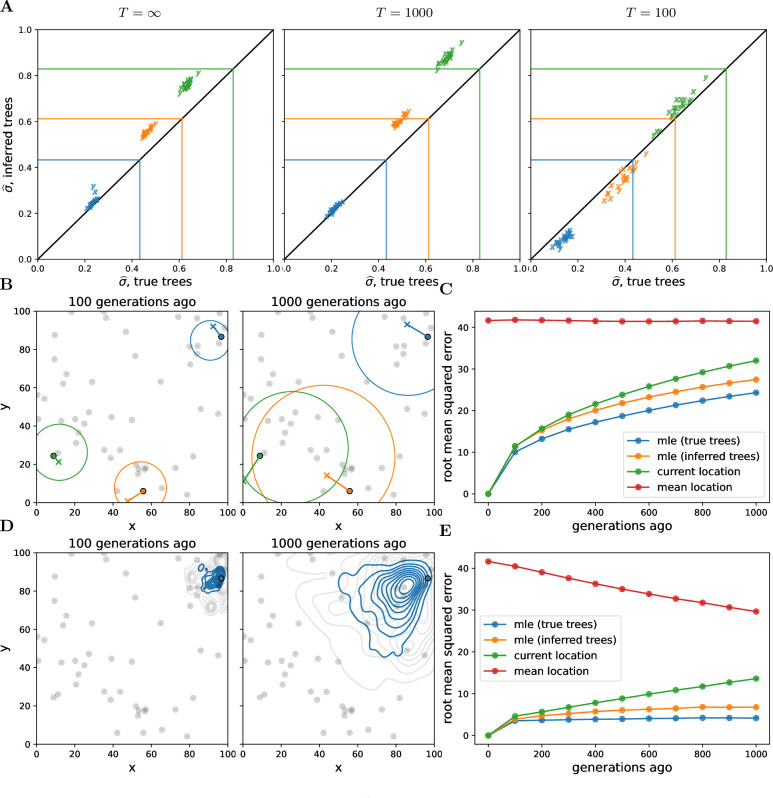
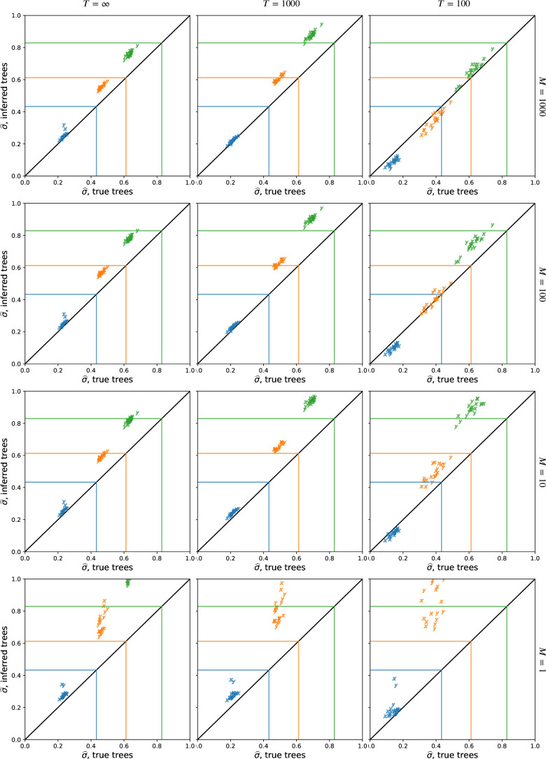
Figure 2—figure supplement 1. The effect of importance sampling on dispersal estimates.

Importance sampling more trees, ${\displaystyle M}$, at each locus brings the dispersal estimate from the inferred trees closer to the dispersal estimate from the true trees and lowers the variance in dispersal estimates across replicates. See Figure 2 for more information, where ${\displaystyle M=1000}$ (top row).

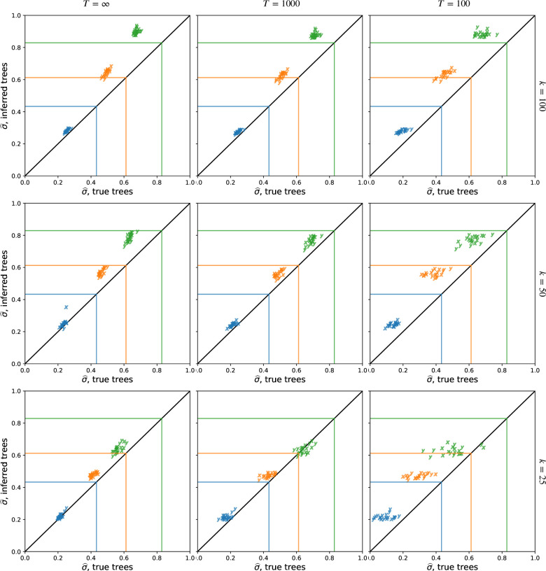
Figure 2—figure supplement 2. The effect of sample size on dispersal estimates.

Using more samples, ${\displaystyle k}$, tends to increase the dispersal estimate from both true and inferred trees and reduce the variation in estimates across replicates at smaller cutoff times. See Figure 2 for more information, where ${\displaystyle k=50}$, ${\displaystyle M=1000}$ and we sample every 100th locus. To isolate the effect of larger trees (rather than more trees), here we use the first ${\displaystyle L=100}$ sampled loci. To speed up calculations, here we use ${\displaystyle M=100}$ importance samples at each locus.

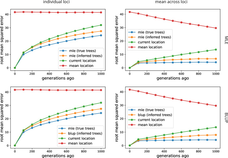
Figure 2—figure supplement 3. Comparing maximum likelihood estimate (MLE) and best linear unbiased predictor (BLUP) ancestor locations.

The top row shows error in the MLE ancestor locations (orange), as in Figure 2, while the bottom row shows the error in the BLUP ancestor locations (orange). The methods are very comparable, though the BLUP method may do slightly worse at estimating the mean ancestor location at deep times.

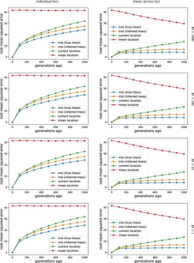
Figure 2—figure supplement 4. The effect of importance sampling on ancestor location estimates.

See Figure 2 for more information, where ${\displaystyle M=1000}$ (top row).

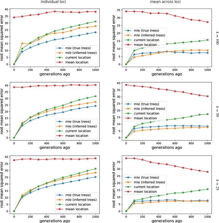
Figure 2—figure supplement 5. The effect of sample size on ancestor location estimates.

See Figure 2 for more information, where ${\displaystyle k=50}$, ${\displaystyle M=1000}$, and we sample every 100th locus. To isolate the effect of larger trees (rather than more trees), here we use the first ${\displaystyle L=100}$ sampled loci. To speed up calculations, here we use ${\displaystyle M=100}$ importance samples at each locus.