

Abstract
Robotic systems rely on spatio-temporal information to solve control tasks. With advancements in deep neural networks, reinforcement learning has significantly enhanced the performance of control tasks by leveraging deep learning techniques. However, as deep neural networks grow in complexity, they consume more energy and introduce greater latency. This complexity hampers their application in robotic systems that require real-time data processing. To address this issue, spiking neural networks, which emulate the biological brain by transmitting spatio-temporal information through spikes, have been developed alongside neuromorphic hardware that supports their operation. This paper reviews brain-inspired learning rules and examines the application of spiking neural networks in control tasks. We begin by exploring the features and implementations of biologically plausible spike-timing-dependent plasticity. Subsequently, we investigate the integration of a global third factor with spike-timing-dependent plasticity and its utilization and enhancements in both theoretical and applied research. We also discuss a method for locally applying a third factor that sophisticatedly modifies each synaptic weight through weight-based backpropagation. Finally, we review studies utilizing these learning rules to solve control tasks using spiking neural networks.
Keywords: Spiking neural networks, Spike-timing-dependent plasticity, R-STDP, Neuromorphic computing, Control problem, Reinforcement learning
Introduction
Robot control systems are extensively researched to meet diverse demands in the robotics industry, covering applications ranging from autonomous vehicle [1] to humanoid robot teleoperation [2], surgical robots [3] and automotive manufacturing [4]. To address the core issue of control in robotic systems, methodologies have significantly evolved from traditional control theories to various deep neural network (DNN)-based approaches, including deep reinforcement learning (DRL) [5]. Traditional methods, typically which rely on sophisticated mathematical models such as proportional-integral-differential (PID) controllers, linear quadratic regulators (LQR), and model predictive control (MPC) for system stability [6], have proven effective in well-defined environments but encounter limitation in handling complex or uncertain systems. The advancement of deep learning models has enabled the successful integration of reinforcement learning (RL) algorithms into the control of complex systems, facilitating interaction with environments characterized by stochastic elements and extensive state and action spaces [7]. Unlike the traditional control theories, the RL models are trained using input data to comprehend the dynamic nature of systems and derive optimal control strategies.
However, addressing control problems in real-world industrial applications requires overcoming the limitations of both robotics and conventional deep learning approaches. In robotics, where a stable energy supply is not always guaranteed, efficient energy consumption is essential [8]. Additionally, short response latency is crucial in control tasks, as robots must continuously collect sensor signals, make decisions, and perform actions. DNN-based approaches, which rely on complex networks with vast numbers of parameters, increase energy consumption and system response latency and may not facilitate high-efficiency control systems. Therefore, to effectively combine the aforementioned constraints of DNNs with the control tasks, developing lightweight models suitable for real-time processing is essential [6].
Spiking neural networks (SNNs), the third-generation artificial neural networks [9] which mimic the functions of the biological brain, originate from the concept [10] and implementation [11] of neuromorphic computing. Unlike the conventional DNNs, SNNs process information based on spikes and temporal dependency, similar to how the human brain transmits and processes information under temporal dynamics. The neuron model of SNNs mimics the principal operations of biological neurons, receiving input spikes through synapses and firing output spikes when the accumulated membrane potential exceeds a threshold. Operating temporally with 1-bit spikes, SNNs excel in modeling real-time data streams, dynamic environments, and evolving patterns over time [12]. Their ability to detect and interpret temporal dynamics in time series data [13] makes them well-suited for control problems requiring real-time and low-power processing. SNNs are appropriate for online learning systems [12], adaptable to unknown environments, and also compatible with neuromorphic hardware [14–16], a type of edge computing. These characteristics suggest that SNNs could create significant synergy when integrated with robotic control systems. This paper reviews the bio-inspired learning rules that fully utilize the temporal dynamics of SNNs and their applications in system control.
From the perspective of artificial intelligence (AI) researchers, algorithm performance remains the primary goal, though considerations of biological plausibility, neuromorphic computing, and other constraints on the reviewed algorithms are also taken into account. Research on neuromorphic computing should be approached from multiple directions [17], and implementing SNNs under these constraints offers the potential to introduce a new paradigm of low-power on-chip computation while preserving key features including temporal dynamics. Spanning from the mathematical modeling of biological brain dynamics [18] to the design of SNNs for the neuromorphic computing [19] and SNNs adopting the existing deep learning architectures [20], several quality reviews [21, 22] have already been presented. Thus, this study focuses on analyzing biologically plausible learning algorithms that are directly relevant to control tasks, without covering neuron models, network topologies, or encoding methods, as these have already been addressed in previous reviews. Additionally, we focus on the compromised biological plausibility, which emphasizes the information propagation and the locality of learning process occurring at the neuron level, without delving down to the molecular and ion channel levels such as neurotransmitters or synapse receptors. The aim is to address the application of the biological learning rules to control tasks, grounded in both theoretical insights and practical experiments.
The sections are organized as follows: Sect. 2 summarizes the implementation of biological learning rules, Sect. 3 describes these rules relative to new factors for large-scale networks, Sect. 4 reviews their applications to control tasks, Sect. 5 discusses open topics for enhancing the performance of learning rules by integrating biological insights with RL algorithms, and Sect. 6 concludes this literature review and discussion.
Bio-inspired learning rule
The concept of bio-inspired learning rules, such as “fire together, wire together," originates from Hebb’s postulate [23], more commonly known as Hebbian learning. This theory emphasizes the causal relationship where the synaptic efficacy between two neurons is strengthened through a process known as the long-term potentiation (LTP) [24] when their spikes fire simultaneously occur in a pre-then-post manner. Conversely, when acausal firings occur, synaptic efficacy weakens, leading to the long-term depression (LTD) [25]. In the context of Hebbian learning, the focus is on the synaptic plasticity in the biological brain, exemplified by spike-timing-dependent plasticity (STDP) [26–28] and Bienenstock-Cooper-Munro (BCM) learning [29]. Additionally, this principle extends to neural networks through rules such as the perceptron learning rule (PLR) [30] and associative memory implemented by the Hopfield network [31]. STDP, which relies on synaptic plasticity driven by the precise spike timing, and BCM, which is based on synaptic plasticity driven by the firing rate are interrelated [32, 33]. As demonstrated in [34], the timing of STDP can be replaced with firing rates that are easily handled by the gradient-based processing. This indicates the potential to connect STDP to the backpropagation learning scheme.
This section primarily focuses on STDP, which is not only supported by extensive biological evidence but is also well-suited for neuromorphic systems. It explores how STDP is applied in the AI field and large-scale systems, gradually building a framework from STDP to the 3-factor rule discussed in Sect. 3. Other forms of biological plasticity, such as depolarization and synaptic cooperativity, along with intrinsic and homeostatic plasticity, are not discussed here as they are covered extensively in other works [35, 36] and fall outside the scope of this paper.
Learning rule for SNN
The unsupervised local learning rule, STDP, is utilized for feature extraction between adjacent layers [37]. Similar to the traditional convolution and activation functions extracting the spatial information, the features extended using STDP contain the information of the firing timing and causality to identify the spatio-temporal patterns, making it suitable for analyzing time series data. However, due to the absence of an explicit objective, STDP faces limitations in deep layer stacking and mathematical optimization. In contrast to DNNs, which adjust all node weights in a supervised manner towards a specific objective, STDP operates in an unsupervised, local, and unbounded manner, creating uncertainty whether the entire network will converge towards the intended objective. To ensure the convergence performance in SNNs, supervised learning and backpropagation-based learning rules have been developed, integrating with DNN frameworks and achieving significant advancements [38, 39]. By leveraging validated models and networks from the DNNs, this approach ensures high performance and has become a popular trend in SNN design.
Early advancements in neuromorphic research, notable advancements in SNNs included SpikeProp [40], known as the first proposal of the backpropagation learning for SNNs, followed by ReSuMe [41], which learns desired timing based on the delta rule, and Tempotron [42], which is trained using the difference between maximum voltage and threshold potential as loss, along with its evolved algorithms [43–45]. To implement the backpropagation learning process for the multi-layer SNNs, Lee et al. [46] designed a differentiable voltage function to compute the membrane potential using auxiliary (pre- and postsynaptic) activity values, while BP-STDP [47] proposed STDP-based backpropagation assuming that the total membrane potential of non-leaky integrate and fire (IF) neurons could be represented by a rectified linear unit (ReLU) activation function. Additionally, Superspike [48] adheres to a temporal window such as STDP and operates as a nonlinear Hebbian three-factor rule. Superspike and STBP [38] proposed SNNs implemented with leaky integrate and fire (LIF) neurons through a recurrent neural network (RNN) structure, combined with a deep learning framework capable of learning through error backpropagation using surrogate functions. Another trend, the ANN-to-SNN conversion [49], was proposed by transforming the ReLU function into IF neurons, offering advantages in absorbing techniques from DNNs, such as Spiking-YOLO [39].
These trends lead to an exclusive exclusive focus on becoming state-of-the-art algorithms with high performance, often neglecting the constraints of neuromorphic systems and the biological foundations as the optimization formula develops, similar to the trajectory of deep learning. However, this approach could endow SNNs with properties akin to DNNs, potentially compromising the unique locality and advantages of SNNs, such as enabling speedy operation for parallel processing in distributed architectures including neuromorphic hardware. Therefore, previously overlooked aspects, particularly focusing on STDP, must be reconsidered to reclaim the unique features of SNNs.
Spike-timing-dependent plasticity
Three features of STDP
From an algorithmic perspective, the basic STDP rule can be divided into three main features: temporal window, causality, and temporal inverse proportionality. The first feature, the temporal window, distinguishes STDP from other synaptic plasticity-based learning methods. Unlike methods that rely on firing frequency [29], depolarization [50] or synaptic activity [34], that is, the STDP learning occurs only when spikes are within a defined temporal window. Figure 1A (i) illustrates the causal STDP [51], where and represent the timings of pre- and postsynaptic spikes, and . The formula for the classical pair-based STDP [28] is as follows:
| 1 |
where w represents the synaptic weight, and and denote the maximum amounts of synaptic modification during LTP and LTD, respectively. and denote the decay constants determining the sensitivity of STDP learning, thereby defining the range of the temporal window. Adjusting these window variables can serve specific purpose without significantly undermining the biological basis. For example, to mitigate the issue of dead neurons caused by LTD during the initial stages of learning, the constant could be set higher than .
Fig. 1.

Various types and implementations of STDP. Red lines represent the potential corresponding to LTP, while blue lines correspond to LTD. A (i) illustrates the typical STDP as adopted from [51], and A (ii) displays its counterpart, that is, the anti-Hebbian STDP. A (iii) illustrates the dopamine (DA)-modulated STDP from [52], where the red lines indicate synaptic changes based on the DA secretion spike intervals, showing a symmetric shape compared to the black control group. A (iv) represents the simplified STDP introduced in [47, 53], where LTP occurs only when the spike interval falls between 0 and . Panel B illustrates the interaction schemes and trace models of STDP. B (i) considers all temporal relationships between spikes, while B (ii) only considers the closest spike. In the trace-based ‘all-to-all’ interaction, spikes accumulate in the trace value, while in the ‘nearest neighbor’ interaction, each spike is replaced by the trace value. Panel C categorizes various types of STDP based on their triggers: C (i) shows the basic pair-based STDP, C (ii) details the postsynaptic spike-driven STDP from [54] where LTP and LTD branches depend on the value, C (iii) illustrates the presynaptic spike-driven STDP from [55] where LTP and LTD occur sequentially with the presynaptic spike’s arrival. If k equals 1, only the latest postsynaptic spike is remembered, leading to inaccurate LTP induction. C (iv) displays the triplet-based STDP from [33], which considers not only the other trace but also its own second trace for more precise synaptic modification
The second feature of STDP, causality, is derived from the Hebbian learning. Anti-Hebbian STDP (aSTDP) illustrated in Fig. 1A (ii) is also considered biologically plausible [56, 57]. In BP-STDP [47], both STDP and aSTDP are employed simultaneously to achieve the desired objectives, and Burbank et al. [58] propose symmetric or mirrored STDP using these two learning models. As illustrated in Fig. 1A (iii) [52], dopamine (DA)-modulated STDP manifests as symmetric STDP. Although the biological plausibility of symmetric STDP is limited to a certain extent, it relies solely on the correlation between pre- and postsynaptic spikes rather than causality, simplifying implementation. As demonstrated by Hao et al. [59], the correlation property of symmetric STDP facilitates the supervised learning without the need for backpropagation by selectively activating target output neurons.
Furthermore, the STDP model exhibits temporal inverse proportionality, where stronger synaptic modifications (high synaptic change in Fig. 1A (i)) occurs when the interval between pre- and postsynaptic spikes is shorter (small in Fig. 1A (i)). However, this feature is not considered in the proposed probabilistic or simplified STDP (sSTDP) [53, 60], which unlike the typical exponential function form of STDP, assumes the form of a rectangular function (Fig. 1A (iv)). This can be expressed by the following equation (Eq. 2), where the same amount of LTP, inversely proportional to the weight, occurs if the spike interval falls within a temporal window of ms, as shown in Fig. 1A (iv).
| 2 |
where LTD occurs with the fixed amount when or . Given that sSTDP is a highly reduced form, BP-STDP [47] using STDP and aSTDP as a type of gate function in a context similar to sSTDP demonstrates high performance. Despite lacking in biological plausibility, sSTDP still remains significant for neuromorphic systems due to its ease of implementation in hardware [53, 61]. Neuromorphic processors should utilize the decayed synaptic changes based on the spike firing times for online learning. However, if a compromising biological plausibility due to the digitalization of the exponential function becomes inevitable, sSTDP could be a viable option. The temporal inverse proportionality depends on the objectives, performance, or computational efficiencies of the STDP designers.
STDP implementation
Upon explaining the principles behind STDP, its various versions have been proposed. Equation 1 represents the additive STDP [28], where synaptic weights converge to upper and lower bounds as learning progresses, forming a bimodal distribution. Since the weights converge to extreme values, this can cause the dead neuron problem while making the model reliant on only a few active neurons during the inference, thereby potentially reducing the generalization of its performance. To transform this extreme distribution into a unimodal one, multiplicative STDP [62] was introduced. In multiplicative STDP, the amplitudes and are replaced by the multiplicative factors and , leading to the following equation:
| 3 |
| 4 |
where denotes the maximum value of w, and and are typically expressed as Eq. 3. In the context of LTP, it is inversely proportional to the synaptic weight w, while LTD is proportional to w, driving the weight toward an intermediate value.
Biological findings [63–65] introduce the concept of synaptic traces, enabling each neuron to accumulate spike history in the trace, facilitating efficient computations. Synaptic traces are calculated by considering the accumulated trace information and spikes at the current time step, without the need to compute all spike temporal relationships within specific intervals. This approach not only enhances the computational efficiency but also makes it suitable for hardware implementation and enables online learning, which is essential for STDP learning. Additionally, the trace allows for the easy implementation of representative interaction schemes such as the ‘all-to-all’ (Fig. 1B (i)) and the ‘nearest neighbor’ (Fig. 1B (ii)) schemes. Equation 5 represents the trace function for the ‘all-to-all’ scheme, allowing both pre- and postsynaptic neurons to record spike history.
| 5 |
where denotes the decay constant for the trace, represents the time when the spike occurred, and the Dirac delta function. Equation 5 represents the simplest trace model, and various trace models with scaling factors applied to the Dirac delta function or adjustments can be found in [65]. When a spike arrives, x(t) becomes the trace function through the nearest spike interaction if it is replaced by (shown in Fig. 1B (ii)) instead of its accumulation of (in Fig. 1B (i)). By adjusting , the STDP temporal window such as and could be controlled. If it is the trace function of the presynaptic neuron, x(t) is updated each time when the presynaptic neuron fires. Additionally, LTP occurs, adjusting the weight in proportion to x(t) each time when the postsynaptic neuron fires. Conversely, if it is the trace function of the postsynaptic neuron, it operates in the opposite manner, causing LTD.
The final and most crucial step in implementing STDP involves determining the criteria to trigger the learning process and the number of spikes required to trigger it. The triggering can be categorized into two types: when either pre- or postsynaptic spikes occur and when both pre- and postsynaptic spikes are fired. Additionally, the spike-based activation for STDP can be categorized into pair- and triplet-based mechanisms. In an advanced implementation, Eq. 4 from the original multiplicative STDP as a trace model is modified to into Eq. 6, refining the model’s adaptability to different synaptic activities and learning conditions.
| 6 |
where and are the trace models of the pre- and postsynaptic neurons, respectively. In the original STDP model, the learning trigger occurs for both post- and presynaptic spikes, as depicted in Fig. 1C (i), where updates to both the weight and the trace occur simultaneously. In contrast, a learning methods proposed by Diehl et al. [54] modifies this approach by recording the presynaptic trace and adjusting weights only upon the arrival of a postsynaptic spike. Equation 7 modified the approach proposed in [54] with subtracting the exponent value for the multiplicative term.
| 7 |
where is the target value, functioning similarly to in Eq. 2, wherein only the target values are lower than the LTP curve (solid line to dashed line in Fig. 1C (ii)), enhancing weights for the immediate follow-up of postsynaptic spike and weakening them for the delayed follow-up.
Another distinct approach is the solo-trigger learning rule, which updates weights exclusively upon the arrival of presynaptic spikes. This presynaptic spike-driven STDP [55, 66, 67] is particularly advantageous for implementation in neuromorphic processors due to its simplicity and the technical constraints often associated with hardware. Specifically, this approach avoids the need for a reverse lookup table, which could be challenging to be implemented due to the memory constraints. In typical hardware setups, the presynaptic neuron is aware of the address of the postsynaptic neuron, but not vice versa. Therefore, without a reverse lookup table, no straightforward method exists for adjusting weights based on postsynaptic activity when only the presynaptic firing information is available. Weights are therefore adjusted only in response to presynaptic spikes arriving. The learning strategy proposed by Park et al. [55] is formulated in the trace model form in Eqs. 8 and 9.
| 8 |
| 9 |
where k denotes the size of the latest spike buffer of the postsynaptic neuron, the arrival time of the latest postsynaptic spike, and the latest postsynaptic trace model. When a presynaptic spike arrives, both the LTP in Eq. 8 and the LTD in Eq. 9 occur sequentially. Unlike LTD, which accurately measures the timing of spikes, LTP’s reliability decreases as the value of k diminishes. Depending on the value of k, several traces of are retained. Figure 1C (iii) depicts how the accuracy of LTP diminishes within the presynaptic spike-driven operation when k is set to 1. There exists a trade-off relationship between memory complexity and LTP accuracy: lower k values reduce memory usage but at the cost of less precise LTP calculations. The authors of [55] claim that their proposed algorithm could reduce the buffer size in neuromorphic chips from 25% to 99% with compared with the previous works.
Triplet-based STDP [33] defines the traditional STDP mechanism by defining the learning rule through the sequences of three spikes-either pre-post-pre or post-pre-post-rather than merely the pair sequences of pre-post or post-pre as seen in pair-based STDP. The utilized parameters are the amplitudes, , , and , and the time constants, , , and . The details are described in Eq. 10 as follows:
| 10 |
| 11 |
where , , and represent the synaptic trace functions, and Eq. 11 illustrates the LTP and LTD through the relationship between the triplet spikes. and represent trace functions similar to those in pairwise STDP, while and represent the trace models reflecting their own intrinsic characteristics. Here, and have the gradually fading-in and fading-out temporal windows compared with and . Figure 1C (iv) illustrates how LTP and LTD are formed through three spikes in the triplet rule.
This triplet rule incorporates twice the number of parameters compared to the conventional pair-based rule, enabling a more comprehensive reflection of biological characteristics. Experimental results [33] have demonstrated that the triplet-based STDP generally outperforms the pairwise approaches in reproducing of the experimental protocols in the visual cortex and hippocampal culture. Beyond the biological reproduction, it is clear that the spatial and temporal complexity in the neuromorphic system increases due to the doubled parameters. Another experiment [68] demonstrated that the triplet STDP exhibited higher pattern recognition in certain conditions compared to its pairwise versions. However, the conclusion emphasizes that triplet STDP might not necessarily be superior to the other forms of STDP but rather serves as a strong candidate.
A concise summary of the equations governing these interactions and adjustments in synaptic plasticity within this subsection 2.2 is compiled in Eq. 12.
| 12 |
The change in synaptic weights is influenced by the timing of pre- and postsynaptic spikes, treated as two input variables in Eq. 12. With variations based on the three key features of STDP-temporal window, causality, and temporal inverse proportionality-and the different implementation methods discussed earlier, STDP models designers have the flexibility to incorporate various STDP functions into Eq. 12. These can range from sSTDP to more complex triplet-based STDP.
Three-factor learning rule
Credit assignment [20, 69, 70] in neural networks is the fundamental process of updating each synaptic weights based on their contribution to network performance, such as total loss or reward. However, STDP primarily relies on two local factors: the presynaptic factor and the postsynaptic factor. These represent the activity or influence of the presynaptic and postsynaptic neurons, respectively, through their spikes, voltage, or a combination of both. The local nature of these factors restricts their ability to adequately assign credit, as they are confined to the synapse between them. This limitation makes it difficult to determine which updates are beneficial at the global network level, especially when stacking layers deeply [19].
To address this limitation, a reward-modulated STDP (R-STDP) has been proposed [71, 72], which incorporates a global reward signal as a third factor along with the local STDP, forming a three-factor learning rule. Unlike the triplet-based STDP mentioned in Sect. 2, which involves three spike events from two local factors, R-STDP utilizes a third factor that is a global modulatory signal. This integration extends the unsupervised STDP into a reward-based learning paradigm, leading to a more comprehensive model of synaptic plasticity that better approximates the temporal dynamics observed in biological nervous systems. Experimental evidence further supports the significant role of neuromodulators in synaptic plasticity, given that dopaminergic neurons transmit widespread signals throughout the brain [73], akin to global reward signals.
This section delineates how to integrate the third factor into the STDP framework to address the credit assignment problem that can be categorized into spatial and temporal aspects. Spatial credit assignment involves distributing credit across the network proportionally to the contributions of individual parameters, as elaborated in Sect. 3.3. By contrast, temporal credit assignment focuses on attributing credit to specific moments when synaptic activities enhance network performance, as discussed in Sects. 3.1 and 3.2.
Eligibility trace for temporal credit assignment
When specific spike patterns induce a reward signal, the synapses contributing to those patterns are eligible for reinforcement. However, as illustrated in Fig. 1A, although the STDP rule is triggered within a few milliseconds, the receipt of the reward may be delayed by seconds or longer. This temporal mismatch introduces the distal reward problem [74], which complicating the assignment of temporal credit to the actions associated with delayed rewards.
To address this challenge, Izhikevich [71] proposed the R-STDP model, which uses an eligibility trace to resolve this issue. Eligibility trace acts as a memory mechanism, recording which neuronal activities are eligible for synaptic updates, thus bridging the temporal gap between the actions and the corresponding rewards. With an index j representing the presynaptic and i representing the postsynaptic neuron, the eligibility trace is defined as follows:
| 13 |
where represents the synaptic memory time constant, and C is the scaling factor of the STDP function as summarized in Eq. 12 from Sect. 2.2. The scaling factor C is crucial since it determines the magnitude of the eligibility trace update. Once accumulated, the eligibility trace value decays slowly, specifically to address the challenge of delayed rewards.
To effectively accommodate delayed rewards, is set to span several seconds, a duration that is significantly longer than the spike trace time constant outlined in Eq. 5. In this equation, the STDP function selects candidates for modification using the trace, rather than instantly updating the weights as in the two-factor STDP rule. Consequently, the temporal credit represented by the eligibility trace enables the backward propagation of reward information; thus, actions closer to the reward are credited more than distant ones, as illustrated in Fig. 2. The update of the synaptic weights, , using the eligibility trace is described as follows:
| 14 |
where M(t) represents a generalized reward concept elaborated in Sect. 3.2. Upon the arrival of the reward, the weights are updated by multiplying the eligibility trace , generalized reward M(t) and learning rate . The learning rate could be gradually decreased [75–77] similar to its application in DNNs.
Fig. 2.
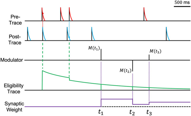
Synaptic weight updates based on to Eq. 14. Inspired by Izhikevich’s work [71]. This figure illustrates the dynamics of synaptic changes. Red lines represent spike traces from presynaptic neurons, while blue lines indicate those from postsynaptic neurons. The eligibility trace, formulated in Eq. 13, is depicted by the green line. The modulator M(t), present at times , , and , modulates the synaptic weight by interacting with the eligibility trace (purple line). Both the pre- and post-traces have a temporal memory span of approximately 100 ms, akin to Fig. 1A, while the eligibility trace has a longer memory duration of approximately 5 s, allowing for delayed rewards. The eligibility trace is dynamically updated through sequential occurrences of LTP and LTD events. At , the weight increases due to the multiplication of the eligibility trace by a positive modulatory factor. At , a negative modulator decreases the weight, and at , the smaller magnitude of the modulator results in only a slight modification to the synaptic weight
Various methods exist for implementing the eligibility trace. In neuromorphic hardware, selecting as a power of two simplifies the implementation, requiring only shifters and adders [78]. Additionally, the eligibility trace functions similarly to a low-pass filter because it acts as a temporal integrator, enabling alternative implementations such as a moving average [79]. This characteristic smooths out fluctuations in the input signal, improving the stability of learning algorithms. Moreover, it aligns well with biological learning mechanisms, providing a bridge between computational models and neural processes. Detailed biological interpretations of the eligibility trace, highlighting its relevance to synaptic plasticity, are well-documented in [80], offering insights into how short-term memories influence long-term learning and adaptation in neural circuits.
Third factors: error, reward, and TD error
Various neuromodulators are being studied as potential candidates for influencing synaptic plasticity. In this section, we introduce modulator M as the third factor in the three-factor learning rule, referred to as modulated-STDP (M-STDP), generalizing its role beyond reward. Modulator M is not limited to a biological perspective and can incorporate any information that guides learning towards solving a downstream task. Although various approaches to designing M-STDP [81], this review focuses on its application through simple multiplication as formulated in Eq. 14.
The modulator M is applied globally yet could selectively enhance the synapses chosen by the STDP rule [82, 83]. Since the modulator M is multiplied by the STDP, it influences the learning speed and even direction when negative values are permitted. As a result, M-STDP resembles the standard STDP with positive rewards (see Fig. 1A (i)), the anti-STDP with negative ones (see Fig. 1A (ii)), and becomes inactive in the absence of rewards. Furthermore, certain studies [52, 84] suggested that the M-STDP could act as the symmetric STDP (see Fig. 1A (iii)). Experimental evidence supports both mechanisms, raising questions regarding the exact role of the modulators in STDP from biological and engineering perspectives. To address this, we emphasize the engineering aspects, refining the classification scheme proposed by Fremaux and Gerstner [81] in this section. We also compare the characteristics of modulator M across various studies focusing on control tasks in Sect. 4. This analysis could enhance the design and utilization of the M-STDP tailored to specific goals and tasks.
Error
The third factor M is derived from biological evidence and the principles of RL. However, for supervised learning tasks with well-defined target-output relationships, formulating M as a supervised error (Eq. 15) could lead to more stable and faster learning, as demonstrated in early studies [85, 86].
| 15 |
where and y denote the predicted output of the network and the supervisory label respectively. The loss function L, chosen based on the task and target data distribution, quantifies the distance between and y. This approach, termed error-modulated STDP (E-STDP), is applicable to control tasks but is constrained by its supervised nature.
Reward
Supervised learning may not be ideal for control tasks where data is dynamically generated through interaction between the agent and the environment, as the model continuously requires labeled data for every action. In such tasks, providing actions as the label due to the stochastic and uncertain nature of the environment is challenging. Instead, using a reward as the modulator could be a more suitable approach. In this case, the modulator is defined as the difference between the actual and expected rewards. Several studies have shown that with repeated conditioning signals and food rewards, the dopaminergic neurons tend to respond more to the conditioning signals than to the rewards [87–91].
When the received reward is less than expected, the neuronal activity decreases, indicating a negative effect due to the actual reward being less than the expected one. This scenario can be generalized using a bias term as shown in Eq. 16
| 16 |
where R represents the actual reward, and b represents a bias term, which is used to adjust the reward by subtracting it from R, effectively acting as the expected reward. The bias b in Eq. 16 quantifies the discrepancy between the actual and the expected rewards. This discrepancy, M, provides insights into how much better or worse certain actions are compared with the expectation. In this context, M functions similarly to an advantage function [92] in RL, which measures the relative benefit of selecting a specific action (by action value function) over others in that state (by state value function). Various studies have used the reward R directly [72, 83], employed a moving average as the bias term [93–95], or scaled it using a sigmoidal function [96].
Temporal difference error
Beyond using statistical expectations or historical reward data to estimate the expected reward in the normalization process, an alternative method predicts the reward, as shown in Eq. 17.
| 17 |
where TD(t) represents the temporal difference (TD) error in RL [7], R the reward received from the environment, and the discount rate that adjusts the value of the next state relative to the value of the current state V(s). Here, s and denote the current and next states, respectively, reflecting the transition dynamics in the environment. This approach requires neurons to serve as the value function, a fundamental component in RL. The value function predicts the state’s value, and is updated by employing the TD error, where the current reward is defined as the difference between the values of the current and next states [97]. To estimate the current reward, the value function takes the current and next states as inputs, and the estimated reward is compared with the actual one obtained from the environment to update the value function. Consequently, the approximation of state values gradually converges to their true value through repeated TD updates [97, 98]. Frémaux et al. [99] introduced TD-STDP, which adopts the continuous time version of the TD error. Employing the TD error as a modulator significantly enhances the learning performance when the value function is incorrect, and the learning process stops when the TD value reaches zero upon convergence.
As discussed earlier, eligibility traces effectively map the delayed rewards to their corresponding neuronal activity, allowing the information to be retained until the delayed rewards arrive. However, if incorrect actions are adopted before the arrival of these delayed rewards, such actions might also be inadvertently reinforced [80]. This complexity renders it challenging to set an appropriate time constant for the eligibility trace, thereby requiring a more precise method to assign temporal credit. In this context, the TD error, calculable at every step, emerges as an alternative that could specifically deal with the challenges associated with sparse and delayed rewards. This approach allows for more precise temporal credit assignment and enables mitigating the issue of reinforcing incorrect actions due to delayed rewards.
Summary
The third factor M could be summarized as follows:
| 18 |
where const indicates that the modulator M operates with a constant value, functioning as the two factor learning rule. E(t), R(t), and TD(t) represent the different frameworks, as previously explained: E(t) denotes the error between predicted and labeled output, R(t) the reward adjusted by subtracting the bias b, and TD(t) the TD error.
Biologically, the third factor might represent various neuromodulators acting in combination. Brzosko et al. [95] proposed a sequential neuromodulated plasticity (SN-Plast) using acetylcholine (ACh) and DA to adjust the parameter used in M-STDP. Their study suggests that the presence of DA induces symmetric STDP (see Fig. 1A (iii)), while ACh without DA leads to a negative value of the symmetric STDP. The system defaults to zero when both are absent. The hybrid approach combining different modulators could be beneficial, and selecting the appropriate modulator based on a specific task and objective is crucial to optimize the learning process.
Synapse-specific modulation for spatial credit assignment
We have investigated the integration of a global modulatory factor into the STDP framework, focusing on temporal credit assignment. The challenge lies in precisely assigning credit to the actions associated with delayed rewards temporally, and to the individual neuron or synapse contributing to the performance spatially. However, most studies fail to allocate spatial credit appropriately; they apply the modulator uniformly across the learning process rather than on a synapse-by-synapse basis. Given that the weights of individual synapses differ, their contributions to the output also vary. Thus, applying the modulator uniformly might result in inaccuracies. Due to these limitations, M-STDP has been applied either to a single layer [78, 100, 101] or uniformly across multiple layers [102]. These approaches take advantage of the relative simplicity of training shallow networks compared to deep ones.
In contrast, the backpropagation algorithm in DNNs [70] has proven effective at accurately allocating spatial credit by calculating the gradient of the loss with respect to each parameter. However, neither the brain nor neuromorphic hardware could implement the differentiation process, which requires considering neuron- or synapse-specific modulation without relying on gradient-based methods [80]. To address this issue, Bing et al. [96] proposed a weight-based backpropagation method. This method distributes the global modulatory signal as localized signals during backpropagation, based on the assumption that larger synaptic weights imply greater contributions of presynaptic neurons to the firing of postsynaptic neurons. As as result, it assigns credit proportionally to the synaptic weights rather than uniformly.
Algorithm 1.

Weight-based Back Propagation
As described in Algorithm 1, the SNN architecture consists of L layers, where each layer, denoted as , is composed of neurons. The reward is assigned for the neuron in the layer. The synaptic weight from this neuron to the neuron in the subsequent layer is represented as . Action neurons in the final layer receive reward directly from the environment, allowing for the customization of rewards for individual action neurons [96]. Neurons in preceding layer receive rewards from neurons in subsequent layer through backpropagation. The reward backpropagated to a single neuron is calculated as the sum of the products of the synaptic weights and their corresponding rewards from connected neurons in the subsequent layer. This sum is normalized by dividing it by the product of the maximum weight value and the number of connected neurons.
Weight-based backpropagation allows for greater diversity in synaptic weights by distributing the credit based on contribution, compared with the uniform multiplication by the modulator. This method ensures superior performance without differentiation, rendering it applicable in neuromorphic hardware, unlike the backpropagation in DNNs. As a result, the weight update rule in Eq. 14 can be rewritten using the synapse-specific modulator M, which incorporates each synaptic weight as the second variable:
| 19 |
Control applications
In this section, we explored the current applications of SNNs across various fields, including image classification [76], object tracking [103], object segmentation [104], pattern generation [105], motor control [6], navigation [106] and physiological data analysis [100, 107]. We describe how the aforementioned learning algorithms, namely STDP and three factor rules, are effectively applied to control task. Table 1 summarizes the use of STDP variants in control and classification tasks. The authors have specified the three-factor rule in various ways; however, for consistency, we refer to it as M-STDP throughout Sect. 3, with a detailed classification provided in Table 1. The subsections are divided into STDP, M-STDP with supervised control, and M-STDP within the RL framework. While distinguishing between RL and non-RL in control problems involving deep learning may be challenging, certain previous studies have explicitly combined M-STDP with the RL framework. Accordingly, we have organized them under Sect. 4.3.
Table 1.
Summary of the recent applications of SNNs in the control and classification tasks
| Author year |
Learning rule | Device | Sensor/data | Task | Env. |
|---|---|---|---|---|---|
| Control | |||||
|
Bouganis et al.. [116] 2010 |
Symmetric STDP |
Humanoid robot (iCub) |
Endogenous Random Generator (ERG) |
Control a 4 degree-of-freedom robotic arm |
Real world |
|
Zennir et al. [117] 2015 |
STDP | Mobile robot | External input current vector | Path planning | Custom simulation |
|
Sarim et al. [118] 2016 |
STDP | Two-wheeled differential drive robot | Five ultrasonic sensors | Autonomous robot navigation | Custom simulation |
|
Milde et al. [110] 2017 |
Pre-driven STDP |
Mobile robot (pushBot) |
DVS |
Obstacle avoidance target acquisition |
Real world |
|
D. Rast et al. [103] 2018 |
STDP |
Humanoid robot (iCub) |
DVS | Object-specific attention |
Aquila, real world |
|
Salt et al. [119] 2019 |
STDP |
Unmanned aerial vehicle (UAV) |
DVS | Obstacle avoidance | Real world |
|
Clawson et al. [85] 2016 |
E-STDP |
Insect-scale robot (RoboBee) |
Proximity sensors, on-board IMU |
Obstacle avoidance trajectory-following |
Real world |
|
Shim et al. [86] 2017 |
R-STDP | Mobile robot |
Five ultrasonic sensors, distance sensor and angle sensor |
Collision avoidance navigation trajectories |
Pygame |
|
Mahadevuni et al. [106] 2017 |
R-STDP | Mobile robot | Five ultrasonic sensors |
Obstacle avoidance autonomous navigation |
Allegro |
| Tieck et al. [112] 2019 | E-STDP |
Robotic arm (Universal robot UR5) |
Reference joint angle targets calculated through inverse kinematics |
Target reaching motions with a 6 degree-of-freedom robotic arm) |
Gazebo |
|
Bing et al. [75] 2019 |
M-STDP | Pioneer robot | Six sonar sensors |
Target reaching obstacle avoidance |
V-REP |
|
Bing et al. [96] 2019 |
R-STDP | Snake-like robot | Infrared vision sensor | Target tracking | V-REP |
| Bing et al. [120] 2018 | R-STDP |
Mobile robot (Pioneer P3-DX) |
DVS | Lane keeping | V-REP |
|
Lobov et al. [108] 2020 |
Multiplicative STDP |
LEGO robot |
Two ultrasonic sonars, two touch sensors |
Obstacle-avoidance | Real world |
|
Bing et al. [121] 2020 |
R-STDP |
Mobile robot (Pioneer P3-DX) |
DVS | Lane keeping | V-REP |
|
Jiang et al. [111] 2020 |
R-STDP | Snake-like robot | DVS | Target tracking | NRP |
|
Liu et al. [115] 2021 |
R-STDP | Mobile robot |
A forward distance sensor, two side distance sensors, two angle sensors |
Obstacle avoidance, target tracking |
Custom simulation |
|
Lu et al. [122] 2021 |
R-STDP | Mobile robot | Three ultrasonic sonars | Obstacle avoidance |
Custom simulation, real world |
|
Quintana et al. [123] 2022 |
R-STDP | Mobile robot | Six ultrasonic sonars | Obstacle avoidance | V-REP |
|
Liu et al. [77] 2022 |
R-STDP | Mobile robot | Two ultrasonic sonars | Obstacle avoidance | Real world |
|
Zhao et al. [124] 2022 |
R-STDP |
Drone swarm (RoboMaster Tello Talent) |
Tello vision positioning system | Multi-robot collision avoidance |
Custom simulation, real world |
|
Zhuang et al. [125] 2023 |
R-STDP | Mobile robot | 3D LiDAR | Lane keeping |
CoppeliaSim, CARLA |
|
Van et al. [126] 2023 |
R-STDP |
Mobile robot (TurtleBot) |
Frequency modulated continuous wave rader |
Collision avoidance, obstacle avoidance, target reaching |
Custom simulation, real world |
|
Zhang et al. [102] 2024 |
R-STDP | - | Real operation data in subway | Railway train control | Custom simulation |
STDP
In 2020, Lobov et al. [108] studied the control of a mobile robot using the spatial properties of STDP in self-learning SNNs. They demonstrated this using a LEGO robot equipped with touch sensors and ultrasonic sonar, showcasing its capability to avoid obstacles. Emphasizing the advantages of SNNs for control tasks, they emphasized that these systems do not require the complex optimization methods, such as backpropagation used in DNNs. Through simulations based on the Izhikevich neuron model and the neurotransmitter dynamics model of Tsodyks-Markram, they demonstrated that STDP could effectively utilize synaptic weight dynamics for robot control. This study demonstrates sensory-motor skill learning and the capabilities of designing SNN architecture, emphasizing the importance of the shortest pathway rule to enhance neural pathway efficiency in obstacle navigation. The shortest pathway rule posits that STDP strengthens the shortest neural pathways within the networks while suppressing the alternative longer pathways. This strategy involves a pair of unidirectional neurons subjected to periodic stimulation, where the activation of the first neuron excites the second neuron, leading to firing if the connection strength is adequate. Synaptic weight adjustment are based on the relative timing of pre- and post-synaptic neuron activity, with LTD occurring if the presynaptic neuron fires only with postsynaptic neuron’s trace value, and LTP occurring in the reverse case. Additionally, the multiplicative mechanism determines the amount of modification in inverse proportion to the weight in the case of LTP and in proportion to the weight in the case of LTD. Using the shortest pathway rule to implement a conditional learning mechanism, the SNN receives two types of inputs (conditional and unconditional stimuli) and activates neurons with only the conditional stimulus. Consequently, the robot gradually learns the association between approaching an obstacle (conditional stimulus) and contact events (unconditional stimulus), enabling it to preemptively avoid obstacles. Further details regarding the application, network structure, and learning rules can be found in [108].
Chao et al. [109] present a drone path planning algorithm through SNNs, enabling energy-efficient and collision-free trajectory calculation. The results demonstrate more enhanced obstacle avoidance and smoother paths to the target compared with the rapidly exploring random trees algorithm. Milde et al. [110] introduced a neural architecture that implements reactive obstacle avoidance and target acquisition using ROLLS, a mixed analog/digital neuromorphic processor, and a dynamic vision sensor (DVS). Their study addresses device variability issues found in traditional electronic circuits and proves robustness under various environmental conditions.
M-STDP with supervised control
In 2019, Bing et al. [96] demonstrated the successful application of a multi-layer SNN trained with M-STDP to a snake-like robot, enabling it to effectively solve target tracking problems. One limitation of the STDP learning rule is its typical reliance on a supervisor or past experience. Additionally, the authors reported that the absence of a unified learning rule applicable across multi-layer SNN structure and the ambiguity in information encoding and decoding in SNNs. Consequently, they proposed ‘a method similar to back-propagation’ [111] that back-propagates rewards through all layers of SNNs to regulate each neuron. Based on this learning rule, they suggested a general workflow for implementing the SNNs controller, along with strategies for information encoding and decoding. The controller learns from the training scenarios and handles unknown scenarios with greater accuracy than the traditional SNNs. It also utilized the R-STDP learning rule in deep networks and real-life robotics. The effectiveness of the proposed algorithm was validated through simulations of three tracking scenarios, conducted in a virtual robot experiment platform (V-REP) environment. To refine the SNN controller, they employed a snake-like robot for target-tracking, which was composed of eight joints and nine identical body modules equipped with two wheels. The head module featured an infrared vision sensor for precise target recognition. The target was set to maintain a high temperature, with its surroundings maintained at a similar temperature. The recorded visual data were encoded through a Poisson distribution as the state for M-STDP, the action of moving left or right was implemented using two actor neurons, with rewards attributed to each neuron indicating opposite signs to mimic the agonist–antagonist muscle system. This approach successfully demonstrated the robot’s ability to accurately track targets. The encoding method and the architecture of the target tracking SNN controller are illustrated in Fig. 3.
Fig. 3.

Encoding strategy of an infrared image input and its SNN architecture, as introduced in [96]. The input data from the infrared camera is resized to simplify data processing and then converted into spike form for input to the neural networks. The SNN structure consists of 64 input neurons, with the intensity of each pixel normalized and used to determine the average firing rate of the spike generator encoding the input image. The SNN controller generates steering commands for a snake-like robot. The spike output of the neural networks is interpreted as motor control commands, with the spike signal decoded to control the robot’s slithering locomotion
In a previous study [111], the aforementioned snake robot was extended to a wheel-less 3D version, utilizing visual signals obtained from a DVS as inputs for the robot’s motion controller. The paper also proposed applying M-STDP across multiple layers in a manner similar to backpropagation learning, where rewards were propagated through layers and their weights updated. The study introduced a simplified topology for the SNN structure by separating the connections from the hidden layer to the output layer. This study demonstrates that a multi-layer SNNs with a separated hidden layer outperforms a basic SNN in moving-target tracking for a wheel-less snake robot, providing enhanced robustness and stability. Clawson et al. [85], focused on a flapping robot named RoboBee, one of the smallest flying robots to achieve autonomous flight. RoboBee’s control was executed through onboard sensors and actuators. It demonstrated that the SNN-based control model could adapt to external changing conditions in real-time during flight through a reward-modulated Hebbian plasticity mechanism, enabling successful autonomous flight. Bing et al. [75] proposed a method for controlling a target-reaching vehicle using supervised learning in SNNs and M-STDP. The primary challenge was to train two SNN-based sub-controllers to achieve obstacle avoidance and target-approaching behaviors through SL, enabling the vehicle to reach its destination while avoiding obstacles. This approach enabled the robot to reach its target in various scenarios.
M-STDP with RL framework
Tieck et al. [112] conducted experiments using a six-degree of freedom (DoF) robotic arm, exploring movements towards and away from a target, inspired by human learning mechanisms. They focused on the learning process through trial and error and the impact of DA on synaptic efficacy changes. Operating in a simulated environment, their methodology did not rely on predefined trajectories; instead, it utilized an RL framework that identified states, actions, and rewards. This framework adjusts synaptic strengths through DA, thereby affecting the reward system. The experimental design involved maneuvering the robotic arm to specified targets by integrating the inverse kinematics (IK) with the SNN model. The reference joint values used for training the agent were generated through a combination of IK calculations and random reaching motions. IK was employed solely for the data generation, not for the actual operation of the agent. Each joint has two states, one when the current joint value is greater than the reference joint value, and the other when it is smaller than the reference joint value. These were represented within the SNNs by two sensory neuron populations. Actions were determined by comparative spike counts in both action neuron populations (up and down), adjusting the joint angle () for subsequent movement. Activations in these neuron populations were modulated with varying DA levels within the synapses for the online learning. The framework incorporates three reward functions for advancing towards the target, retreating from it and ceasing the learning process, thereby preserving the synaptic weights after a period of adaptation. Reward allocation depended on the distance deviation between the robot’s current position and the target across consecutive simulation steps. A reward was designed to reduce this distance, indicating the progress toward the target, while a reward , allocated to increase the distance, moving away from the target. The policy, which determines the action to be selected, was encoded in the synaptic weights between the sensory and action populations. Additionally, a function was implemented to halt the training process, thereby preserving the existing synaptic weights after a predefined learning period. This approach not only enabled a goal-oriented movement but also allowed for the fine-tuning of the robot’s learning process based on task requirements. In conclusion, the study conducted by Tieck et al. presented a methodology for controlling robotic arms with using RL and SNNs. The combination of RL and SNNs, their research has shown promising results in dealing with the complexities of robotic control, particularly in systems with high DoF (Fig. 4).
Fig. 4.
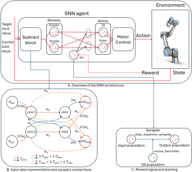
SNN architecture for single-joint control of a robotic arm, introduced by Tieck et al. [112]. a Sensory neurons are stimulated by the difference between the current joint angle and the target angle. Two groups of neurons, one for greater values and one for smaller values, determine the action based on the difference between the target and the current joint value. Action and the magnitude of joint movement (up or down) is determined by comparing the number of spikes of the neuron population responsible for each action. b The current joint angle () and target position () are represented by two sensory populations. The synchronizer network (sync) receives N different inputs and synchronizes their first encoding spikes in the output end [113]. The output spike from sync1 leads to the excitation of inb1 and the inhibition of inb2, while the output from sync2 leads to the excitation of inb2 and the inhibition of inb1. Positive () and negative () neurons are connected to the sensory populations, the former corresponding to angles smaller than the target and the latter for angles greater than the target. Excitatory synapses () are denoted in orange, and inhibitory synapses () are represented in blue. c When a reward signal is present, the activation of DA populations influences STDP, triggering the learning process and the adaptation of the synaptic weights. The NEST simulator was used to model this mechanism with the stdp_dopamine_synapse model employed for the connections between the sensory and action populations [71, 114]. A key aspect of this implementation is that a neuronal population is directly connected to a synapse, rather than another population, using the volume_transmitter interface
Liu et al. [115] introduced a multi-task learning approach for a mobile robot, utilizing a single distance sensor for both obstacle avoidance and target tracking in real environment rather than a simulation. They proposed a task switching mechanism that dynamically alters its lateral inhibition structure in response to variations in firing rates of input spikes, initiated based on the proximity to obstacles and the orientation to a target. The firing frequency of input spikes increases as the robot approaches an obstacle, as detected by the distance sensor, generating a reward signal that inversely correlates with the obstacle proximity. The authors utilized TD error in spike firing frequencies as a learning mechanism, enabling the robot to autonomously learn multiple tasks. This study allowed the SNN-based robot controllers to autonomously learn and execute multiple tasks, demonstrating the potential for advanced learning capabilities in robotic systems.
The brain-inspired controller developed by Zhang et al. [102] aimed to improve the cooperative management and active protection protocols within railway networks. Leveraging empirical data from the Beijing Yizhuang subway line, this approach tried to replicate computational strategies observed in the human brain’s neural architecture, effectively tackling challenges such as real-time train velocity monitoring, coordination, and active protection mechanisms. The controller processes the system’s states, obtained by the train’s real-time information including position, velocity, and relative distance to the preceding train, which is processed by the controller. The learning process is guided by a reward mechanism in the form of DA, which initiates synaptic modifications through the STDP mechanism. This process dynamically adjusts the synaptic weights in the networks, fostering agile adaptation to the train’s operational performance in alignment with predefined objectives and safety parameters. Successful actions, indicated by an increase in DA signal, encourage the strength of advantageous synaptic connections via LTP. Conversely, unsuccessful outcomes lead to a decrease in DA signals, affecting the weakening synapses through LTD and thereby discouraging ineffective behaviors. The networks process the inputs related to the train speed and location, converting them into spike trains using a Poisson distribution. Subsequently, network outputs are transformed into continuous signals that manage the train’s traction and braking systems, employing sigmoid functions for the normalization of the decoded outputs. Zhang et al. have proposed an innovative neurologically inspired strategy to enhance collaborative control and safety measures. They highlight the necessity of continued exploration into the complex challenges and biological features in forthcoming studies.
Discussion
In the previous sections, we explored STDP rules and their variations, including M-STDP, in the context of enhancing performance. Despite substantial efforts in both biological and practical domains to improve these learning rules, approaches to allocating more precise credit still require further research.
The shift in modulators from error to reward and TD error, was inspired by the RL framework. This section explores the incorporation of various elements from the RL paradigm into STDP, highlighting the advantages of integrating RL with STDP by comparing their characteristics. Firstly, both RL and STDP are grounded in biological backgrounds. RL potentially relates to the biological brain, as it is inspired by rewarded behavior in the animal learning process, while STDP directly models the synaptic plasticity occurring within the brain. Secondly, RL has been widely applied to sequential control problems, particularly in robotics, where energy efficiency and rapid response are crucial. These requirements align with the advantages of utilizing STDP. Moreover, the ability of SNNs to manage temporal dynamics enables the processing of time-varying signals in sequential control problems. Thirdly, integrating RL and STDP could help address the learning instability often encountered in RL algorithms, which stems from their exploratory nature and sensitivity to parameter configurations. SNNs, known for their robustness, could provide a complementary approach to these challenges. Finally, STDP, an unsupervised learning framework, could be enhanced by the incorporation of RL elements such as reward and TD error.
Intrinsic motivation
As explained in Sect. 3.2, employing TD error as a modulator has shown promise in environments characterized by delayed and sparse rewards. This approach enables incremental learning by predicting the rewards at each step. However, in scenarios where rewards are absent, or difficult to design, intrinsic motivation (IM) could be a valuable consideration. Analogous to unsupervised learning, which addresses tasks without explicit labels utilized in supervised learning, RL tasks without clear rewards could benefit from leveraging IM for effective problem-solving.
IM can be implemented in various ways, each focusing on different aspects of the agent’s learning process. One approach is to implement IM based on knowledge acquisition, motivating the agent to explore and learn about new aspects of the environment. This could be measured using novelty or information gain achieved by the agent’s actions. Novelty is high when a significant discrepancy exists between the agent’s predictive model and the observed environment. The information gain, defined as the difference in information entropy of the agent’s belief state before and after taking an action, quantifies the reduction in uncertainty or the increase in knowledge regarding the environment. Such approaches could improve exploration in environments with sparse or even absent rewards. Another approach to implementing IM is through skill learning, which involves the agent’s ability to construct task-independent and reusable skills. This approach has two core components: learning a representation of diverse skills and intelligently selecting which skills to learn through a curriculum. By focusing on skill learning, the agent is intrinsically motivated to develop an abstract understanding of skills and to select the most appropriate skills to learn. Unlike knowledge acquisition-based IM, which emphasizes gaining environmental knowledge, skill learning-based IM focuses on the development and selection of skills. Given these possibilities, IM as a modulator presents a promising avenue for future research. For a more detailed discussion on IM, refer to [127].
Multiple modulation
As demonstrated in SN-plast, mentioned in Sect. 3.3, utilizing multiple modulators offers another promising strategy. For example, in the actor-critic structure of RL, different modulators could be assigned to the actor and critic networks. The actor networks, responsible for deciding actions that lead to receiving rewards from the environment, are well-suited to use reward as a modulator. Critic networks, which update the value function using TD error, are appropriate for TD error modulation.
Building on this concept, different modulators for distinct objectives in cases involving multiple actors [128] or multiple agents [129] are also worth considering. For networks expected to engage in greater exploration, IM could be used as a modulator. The magnitude of IM increases with the uncertainty of the environment, leading to larger parameter changes. This approach encourages exploration in uncertain environments, allowing the network to collect more information and potentially discover better strategies. By assigning different modulators to networks with distinct roles, the learning process could allow for a more specialized and efficient adaptation to the RL system in the complex and dynamic environments encountered by each component.
Improved weight-based backpropagation
In Sect. 3.3, a weight-based backpropagation method was introduced, which assumes that a neuron’s contribution to a specific action is determined by its synaptic weight. However, this assumption could be refined to incorporate the frequency of the presynaptic neuron’s firing. For an action neuron in the output layer to fire, its presynaptic neurons must transmit action potentials through spikes. Consequently, the contribution of each presynaptic neuron depends not only on the synaptic weight, which is multiplied by the spike transmission, but also on the firing frequency of the presynaptic neuron. This implies that both the synaptic weight and the presynaptic neuron’s firing frequency should be considered when determining the neuron’s contribution to a specific action.
This refined assumption could align with learning rules based on spike frequency such as the BCM rule, which can be mathematically derived from a minimal version of the triplet STDP [33]. Therefore, incorporating the triplet rule into the weight-based backpropagation method would be beneficial for satisfying the assumption regarding neuronal contribution, as it accounts for both synaptic weight and presynaptic neuron firing frequency. This enhancement could lead to more biologically plausible and effective learning in SNNs.
Conclusion
This review explored various studies on brain-inspired learning rules for SNN training, with a particular focus on addressing control problems. Control problems can be efficiently addressed using SNNs and neuromorphic computing. However, many SNN algorithms have adopted methodologies from DNNs, leading to challenges in compatibility with neuromorphic systems and biological plausibility. To address these challenges, this study revisits biological approaches, examining the STDP rule and its enhanced version, M-STDP. STDP has several variations based on its features and implementation methods, which have been structured into a unified framework. Subsequently, research aiming to overcome the limitations of STDP through the utilization of a third factor is discussed. These studies show that the third factor can be implemented not only by rewards but also by losses and TD errors. Additionally, studies introducing weight-based backpropagation have demonstrated that spatial credit assignment can also be addressed using STDP-based rules. Recent research has demonstrated that control tasks could be effectively conducted in both simulated and real environments based on these learning rules. This study highlights the growing body of research leveraging the unique potential of SNNs, which are biologically plausible and enable low-power on-chip learning, rather than directly mimicking deep learning methodologies.
Acknowledgements
This work was supported by the Technology Innovation Program (RS-2024-00154678, Development of Intelligent Sensor Platform Technology for Connected Sensor) funded by the Ministry of Trade, Industry & Energy(MOTIE, Korea), the National Research Foundation of Korea (NRF) grant funded by the Korea government (MSIT) (No. RS-2022-00165231) and Excellent researcher support project of Kwangwoon University in 2024.
Funding
This work was supported by the Technology Innovation Program (RS-2024-00154678, Development of Intelligent Sensor Platform Technology for Connected Sensor) funded by the Ministry of Trade, Industry & Energy(MOTIE, Korea), the National Research Foundation of Korea (NRF) grant funded by the Korea government (MSIT) (No. RS-2022-00165231) and Excellent researcher support project of Kwangwoon University in 2024.
Declarations
Conflict of interest
The authors declare that they have no Conflict of interest.
Ethical approval
This article does not contain any studies with human participants or animals performed by any of the authors.
Consent to participate
This research did not involve human participants, and as such, consent to participate is not required.
Consent to publish
This manuscript does not contain any individual person’s data in any form.
Footnotes
Publisher's Note
Springer Nature remains neutral with regard to jurisdictional claims in published maps and institutional affiliations.
Choongseop Lee, Yuntae Park, Sungmin Yoon, Jiwoon Lee have contributed equally to this work.
Contributor Information
Youngho Cho, Email: yhcho@daelim.ac.kr.
Cheolsoo Park, Email: parcheolsoo@kw.ac.kr.
References
- 1.Jo Y, Hong S, Ha J, Hwang S. Visual slam-based vehicle control for autonomous valet parking. IEIE Trans Smart Process Comput. 2022;11(2):119–25. [Google Scholar]
- 2.Sa J-M, Choi K-S. Humanoid robot teleoperation system using a fast vision-based pose estimation and refinement method. IEIE Trans Smart Process Comput. 2021;10(1):24–30. [Google Scholar]
- 3.Kim M, Zhang Y, Jin S. Soft tissue surgical robot for minimally invasive surgery: a review. Biomed Eng Lett. 2023;13(4):561–9. [DOI] [PMC free article] [PubMed] [Google Scholar]
- 4.Li W, Tang S. Research on the application of intelligent technology based on the vector controller and wireless module in automotive manufacturing. IEIE Trans Smart Process Comput. 2024;13(3):197–208. [Google Scholar]
- 5.Annaswamy AM, Fradkov AL. A historical perspective of adaptive control and learning. Annu Rev Control. 2021;52:18–41. [Google Scholar]
- 6.Bing Z, Meschede C, Röhrbein F, Huang K, Knoll AC. A survey of robotics control based on learning-inspired spiking neural networks. Front Neurorobot. 2018;12:35. [DOI] [PMC free article] [PubMed] [Google Scholar]
- 7.Sutton RS, Barto AG. Reinforcement Learning: An Introduction. Cambridge, MA, USA: MIT press; 2018. [Google Scholar]
- 8.Stagsted R, Vitale A, Binz J, Bonde Larsen L, Sandamirskaya Y, et al. Towards neuromorphic control: A spiking neural network based pid controller for uav.;2020. RSS
- 9.Gerstner W, Kistler WM. Spiking Neuron Models: Single Neurons, Populations. Cambridge: Plasticity. Cambridge University Press; 2002. [Google Scholar]
- 10.Mead C. Neuromorphic electronic systems. Proc IEEE. 1990;78(10):1629–36. [Google Scholar]
- 11.Mahowald M. Vlsi analogs of neuronal visual processing: a synthesis of form and function. PhD thesis, California Institute of Technology Pasadena;1992
- 12.Lobo JL, Del Ser J, Bifet A, Kasabov N. Spiking neural networks and online learning: An overview and perspectives. Neural Netw. 2020;121:88–100. [DOI] [PubMed] [Google Scholar]
- 13.Albrecht DG, Geisler WS, Frazor RA, Crane AM. Visual cortex neurons of monkeys and cats: temporal dynamics of the contrast response function. J Neurophysiol. 2002;88(2):888–913. [DOI] [PubMed] [Google Scholar]
- 14.Furber SB, Galluppi F, Temple S, Plana LA. The spinnaker project. Proc IEEE. 2014;102(5):652–65. [Google Scholar]
- 15.Akopyan F, Sawada J, Cassidy A, Alvarez-Icaza R, Arthur J, Merolla P, Imam N, Nakamura Y, Datta P, Nam G-J, et al. Truenorth: Design and tool flow of a 65 mw 1 million neuron programmable neurosynaptic chip. IEEE Trans Comput Aided Des Integr Circuits Syst. 2015;34(10):1537–57. [Google Scholar]
- 16.Davies M, Srinivasa N, Lin T-H, Chinya G, Cao Y, Choday SH, Dimou G, Joshi P, Imam N, Jain S, et al. Loihi: A neuromorphic manycore processor with on-chip learning. IEEE Micro. 2018;38(1):82–99. [Google Scholar]
- 17.Schuman CD, Kulkarni SR, Parsa M, Mitchell JP, Kay B, et al. Opportunities for neuromorphic computing algorithms and applications. Nature Comput Sci. 2022;2(1):10–9. [DOI] [PubMed] [Google Scholar]
- 18.Gerstner W, Kistler WM, Naud R, Paninski L. Neuronal Dynamics: From Single Neurons to Networks and Models of Cognition. Cambridge: Cambridge University Press; 2014. [Google Scholar]
- 19.Rathi N, Chakraborty I, Kosta A, Sengupta A, Ankit A, Panda P, Roy K. Exploring neuromorphic computing based on spiking neural networks: Algorithms to hardware. ACM Comput Surv. 2023;55(12):1–49. [Google Scholar]
- 20.Eshraghian JK, Ward M, Neftci EO, Wang X, Lenz G, Dwivedi G, Bennamoun M, Jeong DS, Lu WD. Training spiking neural networks using lessons from deep learning. Proceedings of the IEEE;2023
- 21.Ponulak F, Kasinski A. Introduction to spiking neural networks: Information processing, learning and applications. Acta Neurobiol Exp. 2011;71(4):409–33. [DOI] [PubMed] [Google Scholar]
- 22.Yi Z, Lian J, Liu Q, Zhu H, Liang D, Liu J. Learning rules in spiking neural networks: A survey. Neurocomputing. 2023;531:163–79. [Google Scholar]
- 23.Hebb DO. The Organization of Behavior: A Neuropsychological Theory. Hove: Psychology press; 2005. [Google Scholar]
- 24.Bliss TV, Lømo T. Long-lasting potentiation of synaptic transmission in the dentate area of the anaesthetized rabbit following stimulation of the perforant path. J Physiol. 1973;232(2):331–56. [DOI] [PMC free article] [PubMed] [Google Scholar]
- 25.Lynch GS, Dunwiddie T, Gribkoff V. Heterosynaptic depression: a postsynaptic correlate of long-term potentiation. Nature. 1977;266(5604):737–9. [DOI] [PubMed] [Google Scholar]
- 26.Markram H, Lübke J, Frotscher M, Sakmann B. Regulation of synaptic efficacy by coincidence of postsynaptic aps and epsps. Science. 1997;275(5297):213–5. [DOI] [PubMed] [Google Scholar]
- 27.Bi G-q, Poo M-m. Synaptic modifications in cultured hippocampal neurons: dependence on spike timing, synaptic strength, and postsynaptic cell type. J neuroscience. 1998;18(24):10464–72. [DOI] [PMC free article] [PubMed] [Google Scholar]
- 28.Song S, Miller KD, Abbott LF. Competitive hebbian learning through spike-timing-dependent synaptic plasticity. Nat Neurosci. 2000;3(9):919–26. [DOI] [PubMed] [Google Scholar]
- 29.Bienenstock EL, Cooper LN, Munro PW. Theory for the development of neuron selectivity: orientation specificity and binocular interaction in visual cortex. J Neurosci. 1982;2(1):32–48. [DOI] [PMC free article] [PubMed] [Google Scholar]
- 30.Rosenblatt F. The perceptron: a probabilistic model for information storage and organization in the brain. Psychol Rev. 1958;65(6):386. [DOI] [PubMed] [Google Scholar]
- 31.Hopfield JJ. Neural networks and physical systems with emergent collective computational abilities. Proc Natl Acad Sci. 1982;79(8):2554–8. [DOI] [PMC free article] [PubMed] [Google Scholar]
- 32.Izhikevich EM, Desai NS. Relating stdp to bcm. Neural Comput. 2003;15(7):1511–23. [DOI] [PubMed] [Google Scholar]
- 33.Pfister J-P, Gerstner W. Triplets of spikes in a model of spike timing-dependent plasticity. J Neurosci. 2006;26(38):9673–82. [DOI] [PMC free article] [PubMed] [Google Scholar]
- 34.Bengio Y, Mesnard T, Fischer A, Zhang S, Wu Y. Stdp as presynaptic activity times rate of change of postsynaptic activity. arXiv preprint arXiv:1509.05936;2015
- 35.Caporale N, Dan Y. Spike timing-dependent plasticity: a hebbian learning rule. Annu Rev Neurosci. 2008;31:25–46. [DOI] [PubMed] [Google Scholar]
- 36.Markram H, Gerstner W, Sjöström PJ. A history of spike-timing-dependent plasticity. Front synaptic neurosci. 2011;3:4. [DOI] [PMC free article] [PubMed] [Google Scholar]
- 37.Kheradpisheh SR, Ganjtabesh M, Thorpe SJ, Masquelier T. Stdp-based spiking deep convolutional neural networks for object recognition. Neural Netw. 2018;99:56–67. [DOI] [PubMed] [Google Scholar]
- 38.Wu Y, Deng L, Li G, Zhu J, Shi L. Spatio-temporal backpropagation for training high-performance spiking neural networks. Front Neurosci. 2018;12:331. [DOI] [PMC free article] [PubMed] [Google Scholar]
- 39.Kim S, Park S, Na B, Yoon S. Spiking-yolo: spiking neural network for energy-efficient object detection. In Proceedings of the AAAI Conference on Artificial Intelligence. 2020;34(7):11270–7. [Google Scholar]
- 40.Bohte SM, Kok JN, La Poutré JA. Spikeprop: backpropagation for networks of spiking neurons. In: ESANN. 2000;48:419–24. [Google Scholar]
- 41.Ponulak F, Kasiński A. Supervised learning in spiking neural networks with resume: sequence learning, classification, and spike shifting. Neural Comput. 2010;22(2):467–510. [DOI] [PubMed] [Google Scholar]
- 42.Gütig R, Sompolinsky H. The tempotron: a neuron that learns spike timing-based decisions. Nat Neurosci. 2006;9(3):420–8. [DOI] [PubMed] [Google Scholar]
- 43.Ghosh-Dastidar S, Adeli H. A new supervised learning algorithm for multiple spiking neural networks with application in epilepsy and seizure detection. Neural Netw. 2009;22(10):1419–31. [DOI] [PubMed] [Google Scholar]
- 44.Taherkhani A, Belatreche A, Li Y, Maguire LP. Dl-resume: A delay learning-based remote supervised method for spiking neurons. IEEE transactions on neural networks and learning systems. 2015;26(12):3137–49. [DOI] [PubMed] [Google Scholar]
- 45.Florian RV. The chronotron: A neuron that learns to fire temporally precise spike patterns;2012 [DOI] [PMC free article] [PubMed]
- 46.Lee JH, Delbruck T, Pfeiffer M. Training deep spiking neural networks using backpropagation. Front Neurosci. 2016;10:508. [DOI] [PMC free article] [PubMed] [Google Scholar]
- 47.Tavanaei A, Maida A. Bp-stdp: Approximating backpropagation using spike timing dependent plasticity. Neurocomputing. 2019;330:39–47. [Google Scholar]
- 48.Zenke F, Ganguli S. Superspike: Supervised learning in multilayer spiking neural networks. Neural Comput. 2018;30(6):1514–41. [DOI] [PMC free article] [PubMed] [Google Scholar]
- 49.Diehl PU, Neil D, Binas J, Cook M, Liu S-C, Pfeiffer M. Fast-classifying, high-accuracy spiking deep networks through weight and threshold balancing. In: 2015 International Joint Conference on Neural Networks (IJCNN), 2015;pp. 1–8 . IEEE
- 50.Sjöström PJ, Häusser M. A cooperative switch determines the sign of synaptic plasticity in distal dendrites of neocortical pyramidal neurons. Neuron. 2006;51(2):227–38. [DOI] [PMC free article] [PubMed] [Google Scholar]
- 51.Bi G-q, Poo M-m. Synaptic modification by correlated activity: Hebb’s postulate revisited. Annu rev neurosci. 2001;24(1):139–66. [DOI] [PubMed] [Google Scholar]
- 52.Zhang J-C, Lau P-M, Bi G-Q. Gain in sensitivity and loss in temporal contrast of stdp by dopaminergic modulation at hippocampal synapses. Proc Natl Acad Sci. 2009;106(31):13028–33. [DOI] [PMC free article] [PubMed] [Google Scholar]
- 53.Nessler B, Pfeiffer M, Buesing L, Maass W. Bayesian computation emerges in generic cortical microcircuits through spike-timing-dependent plasticity. PLoS Comput Biol. 2013;9(4):1003037. [DOI] [PMC free article] [PubMed] [Google Scholar]
- 54.Diehl PU, Cook M. Unsupervised learning of digit recognition using spike-timing-dependent plasticity. Front Comput Neurosci. 2015;9:99. [DOI] [PMC free article] [PubMed] [Google Scholar]
- 55.Park J, Jung S-D. Presynaptic spike-driven spike timing-dependent plasticity with address event representation for large-scale neuromorphic systems. IEEE Trans Circuits Syst I Regul Pap. 2020;67(6):1936–47. [Google Scholar]
- 56.Bell CC, Han VZ, Sugawara Y, Grant K. Synaptic plasticity in a cerebellum-like structure depends on temporal order. Nature. 1997;387(6630):278–81. [DOI] [PubMed] [Google Scholar]
- 57.Letzkus JJ, Kampa BM, Stuart GJ. Learning rules for spike timing-dependent plasticity depend on dendritic synapse location. J Neurosci. 2006;26(41):10420–9. [DOI] [PMC free article] [PubMed] [Google Scholar]
- 58.Burbank KS. Mirrored stdp implements autoencoder learning in a network of spiking neurons. PLoS Comput Biol. 2015;11(12):1004566. [DOI] [PMC free article] [PubMed] [Google Scholar]
- 59.Hao Y, Huang X, Dong M, Xu B. A biologically plausible supervised learning method for spiking neural networks using the symmetric stdp rule. Neural Netw. 2020;121:387–95. [DOI] [PubMed] [Google Scholar]
- 60.Tavanaei A, Masquelier T, Maida AS. Acquisition of visual features through probabilistic spike-timing-dependent plasticity. In: 2016 International Joint Conference on Neural Networks (IJCNN), 2016;pp. 307–314 . IEEE
- 61.Querlioz D, Bichler O, Dollfus P, Gamrat C. Immunity to device variations in a spiking neural network with memristive nanodevices. IEEE Trans Nanotechnol. 2013;12(3):288–95. [Google Scholar]
- 62.Rubin J, Lee DD, Sompolinsky H. Equilibrium properties of temporally asymmetric hebbian plasticity. Phys Rev Lett. 2001;86(2):364. [DOI] [PubMed] [Google Scholar]
- 63.Cai F, Frey JU, Sanna PP, Behnisch T. Protein degradation by the proteasome is required for synaptic tagging and the heterosynaptic stabilization of hippocampal late-phase long-term potentiation. Neuroscience. 2010;169(4):1520–6. [DOI] [PubMed] [Google Scholar]
- 64.Morrison A, Aertsen A, Diesmann M. Spike-timing-dependent plasticity in balanced random networks. Neural Comput. 2007;19(6):1437–67. [DOI] [PubMed] [Google Scholar]
- 65.Morrison A, Diesmann M, Gerstner W. Phenomenological models of synaptic plasticity based on spike timing. Biol Cybern. 2008;98(6):459–78. [DOI] [PMC free article] [PubMed] [Google Scholar]
- 66.Brader JM, Senn W, Fusi S. Learning real-world stimuli in a neural network with spike-driven synaptic dynamics. Neural Comput. 2007;19(11):2881–912. [DOI] [PubMed] [Google Scholar]
- 67.Serrano-Gotarredona T, Masquelier T, Prodromakis T, Indiveri G, Linares-Barranco B. STDP and STDP variations with memristors for spiking neuromorphic learning systems. Front Neurosci. 2013;7:2. [DOI] [PMC free article] [PubMed] [Google Scholar]
- 68.Krunglevicius D. Modified stdp triplet rule significantly increases neuron training stability in the learning of spatial patterns. Adv Artif Neural Syst. 2016;2016(1):1746514. [Google Scholar]
- 69.Minsky M. Steps toward artificial intelligence. Proc IRE. 1961;49(1):8–30. [Google Scholar]
- 70.Rumelhart DE, Hinton GE, Williams RJ. Learning representations by back-propagating errors nature. 1986;323(6088):533–6. [Google Scholar]
- 71.Izhikevich EM. Solving the distal reward problem through linkage of stdp and dopamine signaling. Cereb Cortex. 2007;17(10):2443–52. [DOI] [PubMed] [Google Scholar]
- 72.Florian RV. Reinforcement learning through modulation of spike-timing-dependent synaptic plasticity. Neural Comput. 2007;19(6):1468–502. [DOI] [PubMed] [Google Scholar]
- 73.Schultz W. Behavioral theories and the neurophysiology of reward. Annu Rev Psychol. 2006;57:87–115. [DOI] [PubMed] [Google Scholar]
- 74.Hull CL. Principles of behavior: an introduction to behavior theory;1943
- 75.Bing Z, Baumann I, Jiang Z, Huang K, Cai C, Knoll A. Supervised learning in snn via reward-modulated spike-timing-dependent plasticity for a target reaching vehicle. Front Neurorobot. 2019;13:18. [DOI] [PMC free article] [PubMed] [Google Scholar]
- 76.Zhou Q, Ren C, Qi S. An imbalanced r-stdp learning rule in spiking neural networks for medical image classification. IEEE Access. 2020;8:224162–77. [Google Scholar]
- 77.Liu J, Hua Y, Yang R, Luo Y, Lu H, Wang Y, Yang S, Ding X. Bio-inspired autonomous learning algorithm with application to mobile robot obstacle avoidance. Front Neurosci. 2022;16: 905596. [DOI] [PMC free article] [PubMed] [Google Scholar]
- 78.He Z, Shi C, Wang T, Wang Y, Tian M, Zhou X, Li P, Liu L, Wu N, Luo G. A low-cost fpga implementation of spiking extreme learning machine with on-chip reward-modulated stdp learning. IEEE Trans Circuits Syst II Express Briefs. 2021;69(3):1657–61. [Google Scholar]
- 79.Legenstein R, Chase SM, Schwartz AB, Maass W. A reward-modulated hebbian learning rule can explain experimentally observed network reorganization in a brain control task. J Neurosci. 2010;30(25):8400–10. [DOI] [PMC free article] [PubMed] [Google Scholar]
- 80.Gerstner W, Lehmann M, Liakoni V, Corneil D, Brea J. Eligibility traces and plasticity on behavioral time scales: experimental support of neohebbian three-factor learning rules. Front neural circuits. 2018;12:53. [DOI] [PMC free article] [PubMed] [Google Scholar]
- 81.Frémaux N, Gerstner W. Neuromodulated spike-timing-dependent plasticity, and theory of three-factor learning rules. Front neural circuits. 2016;9:85. [DOI] [PMC free article] [PubMed] [Google Scholar]
- 82.Loewenstein Y, Seung HS. Operant matching is a generic outcome of synaptic plasticity based on the covariance between reward and neural activity. Proc Natl Acad Sci. 2006;103(41):15224–9. [DOI] [PMC free article] [PubMed] [Google Scholar]
- 83.Legenstein R, Pecevski D, Maass W. A learning theory for reward-modulated spike-timing-dependent plasticity with application to biofeedback. PLoS Comput Biol. 2008;4(10):1000180. [DOI] [PMC free article] [PubMed] [Google Scholar]
- 84.Seol GH, Ziburkus J, Huang S, Song L, Kim IT, Takamiya K, Huganir RL, Lee H-K, Kirkwood A. Neuromodulators control the polarity of spike-timing-dependent synaptic plasticity. Neuron. 2007;55(6):919–29. [DOI] [PMC free article] [PubMed] [Google Scholar]
- 85.Clawson TS, Ferrari S, Fuller SB, Wood RJ. Spiking neural network (snn) control of a flapping insect-scale robot. In: 2016 IEEE 55th Conference on Decision and Control (CDC), 2016;pp. 3381–3388 . IEEE
- 86.Shim MS, Li P. Biologically inspired reinforcement learning for mobile robot collision avoidance. In: 2017 International Joint Conference on Neural Networks (IJCNN), 2017;pp. 3098–3105 . IEEE
- 87.Ljungberg T, Apicella P, Schultz W. Responses of monkey dopamine neurons during learning of behavioral reactions. J Neurophysiol. 1992;67(1):145–63. [DOI] [PubMed] [Google Scholar]
- 88.Montague PR, Dayan P, Sejnowski TJ. A framework for mesencephalic dopamine systems based on predictive hebbian learning. J Neurosci. 1996;16(5):1936–47. [DOI] [PMC free article] [PubMed] [Google Scholar]
- 89.Schultz W, Dayan P, Montague PR. A neural substrate of prediction and reward. Science. 1997;275(5306):1593–9. [DOI] [PubMed] [Google Scholar]
- 90.Schultz W. Predictive reward signal of dopamine neurons. J neurophysiol. 1998;80(1):1–27. [DOI] [PubMed] [Google Scholar]
- 91.Schultz W. Getting formal with dopamine and reward. Neuron. 2002;36(2):241–63. [DOI] [PubMed] [Google Scholar]
- 92.Schulman J, Moritz P, Levine S, Jordan M, Abbeel P. High-dimensional continuous control using generalized advantage estimation. arXiv preprint arXiv:1506.02438;2015
- 93.Frémaux N, Sprekeler H, Gerstner W. Functional requirements for reward-modulated spike-timing-dependent plasticity. J Neurosci. 2010;30(40):13326–37. [DOI] [PMC free article] [PubMed] [Google Scholar]
- 94.Ghaemi H, Mirzaei E, Nouri M, Kheradpisheh SR. Biolcnet: Reward-modulated locally connected spiking neural networks. In: International Conference on Machine Learning, Optimization, and Data Science, 2022;pp. 564–578 . Springer
- 95.Zannone S, Brzosko Z, Paulsen O, Clopath C. Acetylcholine-modulated plasticity in reward-driven navigation: a computational study. Sci Rep. 2018;8(1):9486. [DOI] [PMC free article] [PubMed] [Google Scholar]
- 96.Bing Z, Jiang Z, Cheng L, Cai C, Huang K, Knoll A. End to end learning of a multi-layered snn based on r-stdp for a target tracking snake-like robot. In: 2019 International Conference on Robotics and Automation (ICRA), 2019;pp. 9645–9651 . IEEE
- 97.Sutton RS. Learning to predict by the methods of temporal differences. Mach Learn. 1988;3:9–44. [Google Scholar]
- 98.Watkins CJ, Dayan P. Q-learning Machine learning. 1992;8:279–92. [Google Scholar]
- 99.Frémaux N, Sprekeler H, Gerstner W. Reinforcement learning using a continuous time actor-critic framework with spiking neurons. PLoS Comput Biol. 2013;9(4):1003024. [DOI] [PMC free article] [PubMed] [Google Scholar]
- 100.Amirshahi A, Hashemi M. Ecg classification algorithm based on stdp and r-stdp neural networks for real-time monitoring on ultra low-power personal wearable devices. IEEE Trans Biomed Circuits Syst. 2019;13(6):1483–93. [DOI] [PubMed] [Google Scholar]
- 101.Akl M, Sandamirskaya Y, Ergene D, Walter F, Knoll A. Fine-tuning deep reinforcement learning policies with r-stdp for domain adaptation. In: Proceedings of the International Conference on Neuromorphic Systems 2022, 2022;pp. 1–8
- 102.Zhang Z, Song H, Wang H, Tan L, Dong H. A novel brain-inspired approach based on spiking neural network for cooperative control and protection of multiple trains. Eng Appl Artif Intell. 2024;127: 107252. [Google Scholar]
- 103.Rast AD, Adams SV, Davidson S, Davies S, Hopkins M, Rowley A, Stokes AB, Wennekers T, Furber S, Cangelosi A. Behavioral learning in a cognitive neuromorphic robot: An integrative approach. IEEE Trans Neural Netw Learn Syst. 2018;29(12):6132–44. [DOI] [PubMed] [Google Scholar]
- 104.Parameshwara CM, Li S, Fermüller C, Sanket NJ, Evanusa MS, Aloimonos Y. Spikems: Deep spiking neural network for motion segmentation. In: 2021 IEEE/RSJ International Conference on Intelligent Robots and Systems (IROS), 2021;pp. 3414–3420 . IEEE
- 105.Lele A, Fang Y, Ting J, Raychowdhury A. An end-to-end spiking neural network platform for edge robotics: From event-cameras to central pattern generation. IEEE Trans Cognit Dev Sys. 2021;14(3):1092–103. [Google Scholar]
- 106.Mahadevuni A, Li P. Navigating mobile robots to target in near shortest time using reinforcement learning with spiking neural networks. In: 2017 International Joint Conference on Neural Networks (IJCNN), 2017;pp. 2243–2250 . IEEE
- 107.Balakrishnan P, Baskaran B, Vivekanan S, Gokul P. Binarized spiking neural networks optimized with color harmony algorithm for liver cancer classification. IEIE Trans Smart Process Comput. 2023;12(6):502–10. [Google Scholar]
- 108.Lobov SA, Mikhaylov AN, Shamshin M, Makarov VA, Kazantsev VB. Spatial properties of stdp in a self-learning spiking neural network enable controlling a mobile robot. Front Neurosci. 2020;14:88. [DOI] [PMC free article] [PubMed] [Google Scholar]
- 109.Chao Y, Augenstein P, Roennau A, Dillmann R, Xiong Z. Brain inspired path planning algorithms for drones. Front Neurorobot. 2023;17:1111861. [DOI] [PMC free article] [PubMed] [Google Scholar]
- 110.Milde MB, Blum H, Dietmüller A, Sumislawska D, Conradt J, Indiveri G, Sandamirskaya Y. Obstacle avoidance and target acquisition for robot navigation using a mixed signal analog/digital neuromorphic processing system. Front Neurorobot. 2017;11:28. [DOI] [PMC free article] [PubMed] [Google Scholar]
- 111.Jiang Z, Otto R, Bing Z, Huang K, Knoll A. Target tracking control of a wheel-less snake robot based on a supervised multi-layered snn. In: 2020 IEEE/RSJ International Conference on Intelligent Robots and Systems (IROS), 2020;pp. 7124–7130 . IEEE
- 112.Tieck JCV, Becker P, Kaiser J, Peric I, Akl M, Reichard D, Roennau A, Dillmann R. Learning target reaching motions with a robotic arm using brain-inspired dopamine modulated stdp. In: 2019 IEEE 18th International Conference on Cognitive Informatics & Cognitive Computing (ICCI* CC), 2019;pp. 54–61 . IEEE
- 113.Lagorce X, Benosman R. Stick: spike time interval computational kernel, a framework for general purpose computation using neurons, precise timing, delays, and synchrony. Neural Comput. 2015;27(11):2261–317. [DOI] [PubMed] [Google Scholar]
- 114.Diesmann M, Gewaltig M-O. Nest: An environment for neural systems simulations. Forschung und wisschenschaftliches Rechnen, Beiträge zum Heinz-Billing-Preis. 2001;58:43–70. [Google Scholar]
- 115.Liu J, Lu H, Luo Y, Yang S. Spiking neural network-based multi-task autonomous learning for mobile robots. Eng Appl Artif Intell. 2021;104: 104362. [Google Scholar]
- 116.Bouganis A, Shanahan M. Training a spiking neural network to control a 4-dof robotic arm based on spike timing-dependent plasticity. In: The 2010 International Joint Conference on Neural Networks (IJCNN), 2010;pp. 1–8 . IEEE
- 117.Zennir MN, Benmohammed M, Boudjadja R. Spike-time dependant plasticity in a spiking neural network for robot path planning. In: AIAI Workshops, 2015;pp. 2–13
- 118.Sarim M, Schultz T, Jha R, Kumar M. Ultra-low energy neuromorphic device based navigation approach for biomimetic robots. In: 2016 IEEE National Aerospace and Electronics Conference (NAECON) and Ohio Innovation Summit (OIS), 2016;pp. 241–247 . IEEE
- 119.Salt L, Howard D, Indiveri G, Sandamirskaya Y. Parameter optimization and learning in a spiking neural network for uav obstacle avoidance targeting neuromorphic processors. IEEE trans neural netw learn syst. 2019;31(9):3305–18. [DOI] [PubMed] [Google Scholar]
- 120.Bing Z, Meschede C, Huang K, Chen G, Rohrbein F, Akl M, Knoll A. End to end learning of spiking neural network based on r-stdp for a lane keeping vehicle. In: 2018 IEEE International Conference on Robotics and Automation (ICRA), 2018;pp. 4725–4732 . IEEE
- 121.Bing Z, Meschede C, Chen G, Knoll A, Huang K. Indirect and direct training of spiking neural networks for end-to-end control of a lane-keeping vehicle. Neural Netw. 2020;121:21–36. [DOI] [PubMed] [Google Scholar]
- 122.Lu H, Liu J, Luo Y, Hua Y, Qiu S, Huang Y. An autonomous learning mobile robot using biological reward modulate stdp. Neurocomputing. 2021;458:308–18. [Google Scholar]
- 123.Quintana FM, Perez-Peña F, Galindo PL. Bio-plausible digital implementation of a reward modulated stdp synapse. Neural Comput Appl. 2022;34(18):15649–60. [Google Scholar]
- 124.Zhao F, Zeng Y, Han B, Fang H, Zhao Z. Nature-inspired self-organizing collision avoidance for drone swarm based on reward-modulated spiking neural network. Patterns 2022;3(11) [DOI] [PMC free article] [PubMed]
- 125.Zhuang G, Bing Z, Zhou Z, Yao X, Huang Y, Huang K, Knoll A. An energy-efficient lane-keeping system using 3d lidar based on spiking neural network. In: 2023 IEEE/RSJ International Conference on Intelligent Robots and Systems (IROS), 2023;pp. 4763–4769 . IEEE
- 126.Van Damme L, Durodié Y, Deckers L, Tsang J, Latré S. Collision avoidance navigation with radar and spiking reinforcement learning. In: 2023 IEEE International Radar Conference (RADAR), 2023;pp. 1–6 . IEEE
- 127.Aubret A, Matignon L, Hassas S. A survey on intrinsic motivation in reinforcement learning. arXiv preprint arXiv:1908.06976;2019 [DOI] [PMC free article] [PubMed]
- 128.Mnih V, Badia AP, Mirza M, Graves A, Lillicrap T, Harley T, Silver D, Kavukcuoglu K. Asynchronous methods for deep reinforcement learning. In: International Conference on Machine Learning, 2016;pp. 1928–1937 . PMLR
- 129.Claus C, Boutilier C. The dynamics of reinforcement learning in cooperative multiagent systems. AAAI/IAAI. 1998;1998(746–752):2. [Google Scholar]