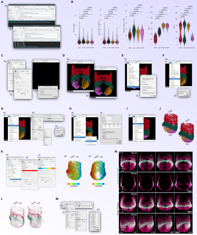
Figure 8.

Dataset Visualization

(A) Plotting Displacement (Steps 67): Scripts to plot peak displacement for tissue-specific data from the SVF dataset.

(B) Plotting Additional Features (Step 68): Generating plots for various track features such as cell density and average velocity.

(C) MaMuT Data Visualization (Step 69): Opening SVF tracking results in MaMuT and adjusting settings for optimal viewing.

(D) 3D Rendering Initialization (Step 69e): Setting up and starting 3D renderings of the SVF tracking data in MaMuT’s 3D Viewer.

(E) Adjusting 3D Viewer Settings (Step 69f): Configuring 3D Viewer dimensions and verifying orientation for accurate visualization.

(F) Animation Setup (Step 70a): Configuring animation settings for creating rotational 3D renderings of the dataset.

(G) Recording and Saving Animation (Step 70b–d): Recording spinning animations of the dataset and saving as an .avi movie file.

(H) Specimen Reorientation (Step 70f): Applying transformations to reorient the specimen for preferred 3D visualization.

(I) Snapshot Capture (Step 70g): Taking and saving snapshots from the 3D Viewer for static visual presentations.

(J) Additional Snapshots (Step 70h): Capturing further views and orientations as still images.

(K) Color Adjustments by Z (Step 70h): Adjusting spot colors in the 3D Viewer based on Z coordinates to enhance depth perception.

(L) Track Visualization in 3D Viewer (Step 70i): Visualizing and processing tracks in a new 3D Viewer session for detailed analysis.

(M) Creating Time Lapse Montages (Step 71a–b): Generating montages from time-lapse .avi files to visualize temporal changes.

(N) Final Montage Adjustments (Step 71c): Finalizing and saving montage presentations, ensuring accurate scale and time representations.