Protein Coding Sequence Identification by Simultaneously Characterizing the Periodic and Random Features of DNA Sequences

Abstract

Most codon indices used today are based on highly biased nonrandom usage of codons in coding regions. The background of a coding or noncoding DNA sequence, however, is fairly random, and can be characterized as a random fractal. When a gene-finding algorithm incorporates multiple sources of information about coding regions, it becomes more successful. It is thus highly desirable to develop new and efficient codon indices by simultaneously characterizing the fractal and periodic features of a DNA sequence. In this paper, we describe a novel way of achieving this goal. The efficiency of the new codon index is evaluated by studying all of the 16 yeast chromosomes. In particular, we show that the method automatically and correctly identifies which of the three reading frames is the one that contains a gene.

INTRODUCTION

Gene identification is one of the most important tasks in the study of genomes. In order to be successful, a gene-finding algorithm has to incorporate good indices for the protein coding regions. In the past two decades, a number of useful codon indices have been proposed. They include the codon bias index (CBI) (Bennetzen and Hall [1]), the codon adaptation index (CAI) (Sharp and Li [2]; Jansen et al [3]), the YZ score (Zhang and Wang [4]), measures based on differences in codon usage (Staden and McLachlan [5]), hexamer counts (Claverie and Bougueleret [6]; Farber et al [7]; Fickett and Tung [8]), codon position asymmetry (Fickett [9]), autocorrelations and nucleotide frequencies (Shulman et al [10]; Fickett [9]; Borodovsky et al [11]), entropy (Almagor [12]), and periodicities, especially the period-3 feature of a nucleotide sequence in the coding regions (Fickett [9]; Silverman and Linsker [13]; Chechetkin and Turygin [14]; Tiwari et al [15]; Trifonov [16]; Yan et al [17]; Anastassiou [18]; Issac et al [19]; Kotlar and Lavner [20]). Most of them mainly capture the feature of highly biased nonrandom usage of codons in the coding regions. The background of a DNA sequence, be it a coding or noncoding sequence, however, is fairly random. Consequentially, a DNA sequence can be characterized as a random fractal. Is it possible to develop a new codon index by simultaneously incorporating the fractal and periodic features of a DNA sequence? The aim of this paper is to develop a simple method to achieve such a goal. Since the codon index obtained this way complements existing codon indices, it has the potential of being incorporated into existing gene identification algorithms so that the accuracy of those algorithms can be improved and their training be simplified.

The novel codon index proposed here is based on two incompatible features of DNA sequences: the period-3 and the fractal features. It has been known for a while that a DNA sequence exhibits fractal properties, with noncoding regions often possessing, but coding regions often lacking long-range correlations (Li and Kaneko [21]; Peng et al [22]; Voss [23]). Roughly speaking, a fractal means a part is similar to another part or to the whole, and hence, does not possess any well-defined scale (Mandelbrot [24]). However, it has been recognized that the biased nonrandom use of codons in coding regions often defines a period-3 feature in the coding regions. Period-3 is a specific scale and hence, is incompatible with the concept of fractal. We show here that a convenient codon index can be developed by exploiting this incompatibility. This is achieved by quantifying the deviation of a DNA sequence from its fractal behavior due to the period-3 feature. Amazingly, this simple measure not only correlates well with coding regions, but also automatically and correctly identifies which of the three reading frames is the correct one (ie, containing a gene). In this paper, we will illustrate the idea and evaluate the proposed index by studying all of the 16 yeast chromosomes.

DATABASES AND METHODS

Database

The yeast chromosome sequences and the associated annotation data used for the analysis are based on sequence dated 1 October 2003 in the Saccharomyces Genome Database (http://www.yeastgenome.org) and can be obtained from ftp://genome-ftp.stanford.edu/pub/yeast/data_download.

The period-3 feature

The period-3 feature of a DNA sequence has been used to develop important codon indices (Fickett [9]; Silverman and Linsker [13]; Chechetkin and Turygin [14]; Tiwari et al [15]; Trifonov [16]; Yan et al [17]; Anastassiou [18]; Issac et al [19]; Kotlar and Lavner [20]). The existence of this feature can be shown, for example, by Fourier spectral analysis. In order to apply Fourier transform, first one has to obtain one or more numerical sequences from a DNA sequence. A common mapping scheme is to construct four binary sequences from a DNA sequence, one for each base. For instance, when nucleotide base “A” is concerned, a sequence u(n) is assigned 1's at those positions where “A” is present, and 0's otherwise. Take sequence

$$\text{S}=\text{AATCGGCCCCGAT}\left(1\right)$$

as an example. One obtains the following binary sequences:

$$\begin{array}{l}u\left(\text{A}\right)=1100000000010,\\ u\left(\text{C}\right)=0001001111000,\\ u\left(\text{G}\right)=0000110000100,\\ u\left(\text{T}\right)=0010000000001.\end{array}\left(2\right)$$

Such a scheme has been used, for example, by Voss [23] and Kotlar and Lavner [20]. Alternatively, one can obtain numerical sequences using the following mapping rules. (a) C or G → u(n) = +1; A or T → u(n) = −1. This rule suggested by Azbel [25] maps a DNA sequence into a sequence of weak/strong hydrogen bonds. (b) C or T → u(n) = +1; A or G → u(n) = −1. This scheme was proposed by Peng et al [22] and maps a DNA sequence into a sequence of purine/pyrimidine. When a numerical sequence u(n) is obtained, the discrete fourier transform (DFT) can be used to compute its spectrum U(k), which is given by

$$U\left(k\right)=\sum _{n=0}^{N-1}u\left(n\right)e^{\left(-2\pi /N\right)nk},\hspace{0.17em}\hspace{0.17em}\hspace{0.17em}\hspace{0.17em}0\le k\le N-1,\left(3\right)$$

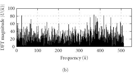
where N is the length of u(n) and k corresponds to the discrete frequency of (2π/N)k or a period of (N/k). U(k) can be conveniently used to identify characteristic periodicities of u(n). Since a coding DNA sequence is comprised of codons (units of three nucleotide bases) and the nucleotide usage in a coding sequence is highly biased and nonrandom, a period of 3 is often present in the coding sequence u(n). This feature is usually referred to as “period-3.” Consequently, the DFT magnitude or power spectrum density of u(n) often displays a distinct peak at k = N/3 (or at a frequency around [N/3] when N/3 is not an integer). However, the period-3 feature is usually lacking or weak in noncoding regions (Fickett [9]; Silverman and Linsker [13]; Chechetkin and Turygin [14]; Tiwari et al [15]; Trifonov [16]; Yan et al [17]; Anastassiou [18]; Issac et al [19]; Kotlar and Lavner [20]). To illustrate this idea, we use Peng's mapping rule to construct u(n) from the coding/noncoding DNA sequences of yeast and perform DFT on u(n) (for simplicity, we have chosen N = 1026). Typical DFT magnitudes |U(k)| for coding and noncoding regions are shown in Figure 1. A strong peak is observed for |U(k)| at k = 1026/3 of the coding region while no such feature is observed for the noncoding region.

Figure 1.

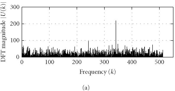
Representative DFT magnitudes for (a) coding and (b) noncoding regions in yeast chromosome I.

Fractal property and the DFA technique

For other analyses, especially fractal analysis, it is more handy to construct a random walk (called DNA walk) from the DNA sequence. The walk y(n) is generated by forming a partial sum of the u(i) sequence constructed from the DNA sequence

$$y\left(n\right)=\sum _{i=1}^{n}u\left(i\right),\hspace{0.17em}\hspace{0.17em}\hspace{0.17em}\hspace{0.17em}n=1,2,3,\dots .\left(4\right)$$

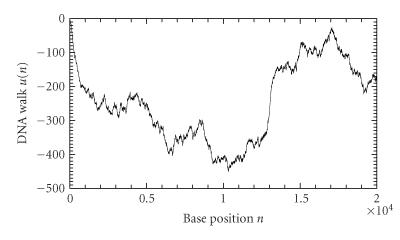
Several different versions of DNA walks have been proposed based on different mapping rules for u(n). The recently proposed 3D DNA walk is also called Z curve (Yan et al [17]; Zhang et al [26]). Note that the DNA walks based on the two 1D mapping rules mentioned above (Azbel [25]; Peng et al [22]) are equivalent to the z-component and x-component of the Z curve, respectively. Other types of multidimensional DNA walks have also been suggested (Berthelsen et al [27]; Cebrat et al [28]). In this work, we will employ the x-component of the Z curve (A or T → u(n) = +1; C or G → u(n) = −1) for further analysis because of its simplicity and efficiency (Stanley et al [29]). An example is shown in Figure 2 for the first 20 000 bases of the chromosome I of yeast. Note that such a mapping generates an equivalent (except differing by a sign) DNA walk for the reverse strand of a DNA sequence. Hence, analysis based on such a mapping processes both strands of a DNA sequence simultaneously.

Figure 2.

An example of a DNA walk constructed from the first 20 000 bases of the chromosome I of yeast.

While DNA walks are useful in many applications, interpretation of some computational results, such as long-range correlations (Stanley et al [29]), are sometimes problematic, due to patchiness effects along a DNA sequence (Karlin and Brendel [30]). To remove such patchiness effects, a method called detrended fluctuation analysis (DFA) was developed by Peng et al [31] and has been used to identify characteristic patch sizes (Viswanathan et al [32]). DFA works as follows: first divide a given DNA walk of length N into ⌊N/l⌋ nonoverlapping segments (where the notation ⌊x⌋ denotes the largest integer that is not greater than x), each containing l nucleotides; then define the local trend in each segment to be the ordinate of a linear least-squares fit for the DNA walk in that segment; finally compute the “detrended walk,” denoted by y_l(n), as the difference between the original walk y(n) and the local trend. The following scaling behavior (ie, fractal property) has been found for many DNA walks studied:

$${\left[F_d\left(l\right)\right]}^2=\langle \sum _{i=1}^l{y}_l{\left(i\right)}^2\rangle \propto l^{2H},\left(5\right)$$

where the angle brackets denote ensemble average of all the segments and F_d(l) is the average variance over all segments. The exponent H is often called the “Hurst parameter” (Mandelbrot [24]). When H = 0.5, the DNA walk is similar to a standard random walk. When H > 0.5, the DNA walk possesses long-range correlations. Statistically speaking, a noncoding region is often more likely to possess the long-range correlation properties (Stanley et al [29]). This feature, together with the DFA technique, was used by Ossadnik et al [33] to develop a coding sequence finder for genomes with long noncoding regions. To further illustrate the ideas, we analyze the coding and noncoding sequences of the yeast genome using the DFA technique. For a coding/noncoding sequence of length N, first a DNA walk y(n) is constructed according to Peng's mapping rule. Then the detrended fluctuation F_d(l) is computed according to (5) for a series of segment sizes l (l < N). In practice, l is often chosen to be the power of a common base r, that is, l(j) = r^j, j = 1,2,..., log_r^N. Notice that log F_d(l) ~ H log l, F_d(l) is approximately linear on double logarithmic scale when l is within a certain range [l₀, l₁]. A linear least-squares fit of data in this range produces a straight line with slope a and intersect b from which we can get an estimate of the Hurst parameter H = a/2. Figure 3 shows a log-log plot of F_d(l) versus l for (a) a coding and (b) a noncoding sequence of yeast chromosome I. The two sequences are of lengths (a) N = 1742 and (b) N = 3598. We choose l to increment with the base r = 2 (also for all following analysis that concerns DFA) and the fitting range with the best scaling property is found to be [l₀, l₁] = [2², 2⁸] for both (a) and (b). Within this range, the Hurst parameters are (a) H = 0.54 and (b) H = 0.62. The nice scaling law in [l₀, l₁] indicates that DNA sequences are fractals. Often, the Hurst parameters in noncoding regions are larger than those in coding regions, suggesting that noncoding regions often possess stronger long-range correlations. Sometimes this feature is termed lesser complexity in noncoding regions (Ossadnik et al [33]; Stanley et al [29]).

Figure 3.

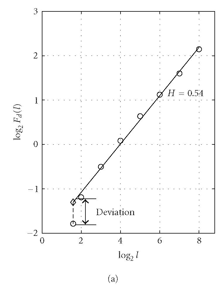
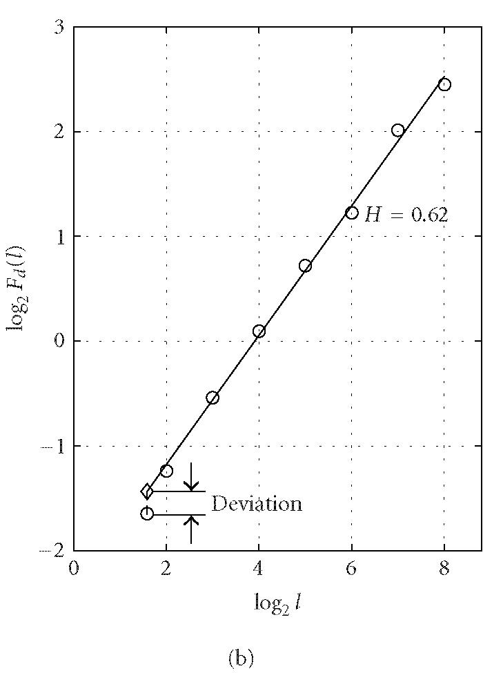
Representative period-3 fractal deviation (PFD) for (a) coding and (b) noncoding regions in yeast chromosome I.

Deviation from fractal scaling due to period-3 signal

Intuitively, when a periodicity exists in a sequence, the fractal scaling law does not hold at that particular “scale” defined by the periodicity. Specifically, for DNA sequences, a normally strong period-3 signal in coding regions causes a “deviation” from the sequence's fractal “background.” On the contrary, for a noncoding region, such deviation, if any, is typically much smaller than that of a coding region. Based on the DFA technique, we have developed a novel codon index which quantifies such deviation from the fractal scaling law due to the period-3 feature, which we will denote by period-3 fractal deviation (PFD) for simplicity.

For a DNA walk y(n) of length N, after computing its detrended fluctuation using DFA and identifying the best fitting range [l₀, l₁], an approximation of F_d(l) can be obtained by

$$log{\hat{F}}_d\left(l\right)=alogl+b.\left(6\right)$$

The deviation of y(n) is defined as the difference between $log{\hat{f}}_d\left(l\right)$ and logF_d(l) at l = 3, that is,

$$\text{PFD}=\left|\text{log}{\hat{F}}_d\left(3\right)-log{F}_d\left(3\right)\right|.\left(7\right)$$

To verify our intuition about the capacity of this index in distinguishing coding and noncoding regions, we have computed the PFD value for a large number of the verified open reading frames (ORFs) and noncoding segments from all of the 16 yeast chromosomes. An example of representative PFD values for coding and noncoding regions is shown in Figure 3. We observe that for the coding region, the fluctuation F_d(l) at l = 3 deviates severely from the power-law relation (ie, the straight line in a log-log plot in Figure 3), while the deviation for the noncoding region is relatively small.

One may wonder if any DNA segment that belongs to a coding region has a large PFD. In fact, this is not the case. The quantification of the period-3 feature by the deviation from fractal scaling is reading-frame dependent. When the coding segment starts with the gene-containing reading frame (the first nucleotide of a codon), the period-3 feature collides with the DFA technique at the scale of l = 3 and results in a large PFD. When the segment starts with an incorrect reading frame, the periodicity of 3 cannot be captured by DFA and the deviation value is small. For noncoding regions where the period-3 feature is usually lacking or weak, the PFD does not change much for the three reading frames. Note that the DFT magnitude for a coding region is similar for all three reading frames while the DFT phase is not. Codon indices based on the latter has improved performance compared with algorithms that use DFT magnitude (Kotlar and Lavner [20]). The PFD measure, whose value also varies for different reading frames, not only quantifies a sequence's coding strength well but also locates the reading frame correctly. The latter statement will be made more concrete shortly.

Algorithm for computing period-3 fractal deviations along a DNA sequence

Based on the observations above, we employ a sliding window technique (with window size w) to calculate PFD along a DNA sequence in a systematic fashion. The algorithm can be stated in four steps.

Step 1. Given a DNA sequence of length N, construct a DNA walk of length N based on the simple purine/pyrimidine rule (Peng et al [22]). Let w be the size of the sliding window. When successive windows overlap by w − 1 bases, a total of N − w + 1 windows can be obtained. For each window, the value of PFD can be computed based on (7).

Step 2. By common sense, one would associate each PFD for a window with the center of the window. In order to preserve information about the reading frames, however, this rule is slightly modified as follows: denote the position of the window along the DNA sequence by [n, n + w − 1]. We associate its PFD with the position n + 3j, where j is the largest integer such that 3j ≤ w/2.

Step 3. Form three reading-frame-specific deviation sequences by dividing the PFD(n) sequence into three subsets, PFD¹(1 + 3m), PFD²(2 + 3m), PFD³(3 + 3m), m = 0, 1, 2, ..., corresponding to the positions (1, 4, 7, ...), (2, 5, 8, ...), (3, 6, 9, ...), respectively. For later convenience, we will denote PFD¹(1 + 3m), PFD²(2 + 3m), PFD³(3 + 3m) by PFD¹(m), PFD²(m), PFD³(m), m = 0, 1, 2, ....

As we will illustrate in the next section, the above three steps automatically exhibit which reading frame is the correct one. Step 4 defines a simple but efficient codon index MAXFD.

Step 4. After PDFⁱ, i = 1, 2, 3 are obtained, we compute

$$\text{MAXFD}=\frac{1}{\lfloor M/3\rfloor }\sum _{m=1}^{\lfloor M/3\rfloor }max\left({\text{PFD}}^{\text{1}}\left(m\right),{\text{PFD}}^{\text{2}}\left(m\right),{\text{PFD}}^{\text{3}}\left(m\right)\right).\left(8\right)$$

Let δ₀ be a threshold value. A segment under study is declared “coding” if the codon index MAXFD is greater than δ₀ and “noncoding” otherwise. In practice, the threshold value δ₀ is usually chosen to be where the cumulative distribution for the coding regions intersects with the complementary cumulative distribution for the noncoding regions (See Figure 4).

Figure 4.

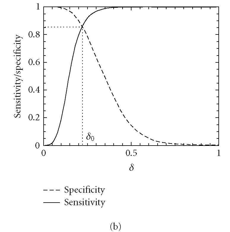
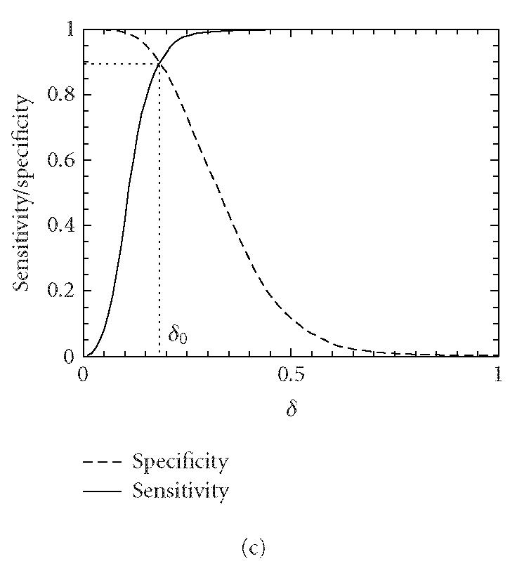
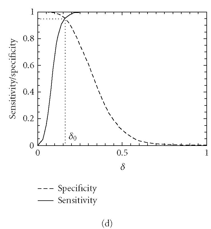
Distributions of MAXFD for the coding (solid curves) and noncoding (dashed curves) subsets of the 16 yeast chromosomes. The sliding window size is w = 512. The parameters n₁ and n₂ designate the coding/noncoding segments with lengths greater than n₁ and n₂, respectively. (a) n₁ = n₂ = 1, (b) n₁ = n₂ = 256, (c) n₁ = n₂ = 512, (d) n₁ = n₂ = 1026. See the text and Table 1 for more details.

RESULTS AND DISCUSSION

The above algorithm has been used to calculate the PFD values of all of the 16 yeast chromosomes. To show that the algorithm is largely independent of the sliding window size as well as to show that the method is applicable to short DNA sequences, sliding window sizes of 128, 256, 512, and 1024 have been tried, with the best scaling regions identified as [2², 2⁴], [2², 2⁵], [2², 2⁶], and [2², 2⁷], respectively. For each window size, after a PFD sequence is obtained for an entire chromosome sequence, the three reading-frame-specific deviation sequences PFDⁱ(m), i = 1, 2, 3, are plotted against their nucleotide positions along the chromosome in red, green, and black, respectively. For all four window sizes, the three deviation curves thus obtained exhibit similar and very interesting patterns. As examples, we have shown in Figures 5 and 6 the three reading-frame-specific PFDⁱ(m) sequences for DNA segments in yeast chromosome I, from nucleotide 58 000 to nucleotide 70 000, and from 141 500 to nucleotide 160 000, respectively, where the window size w is chosen to be 512. To appreciate the correlations between the patterns of the variations of the PFDⁱ(m) sequences and the coding/noncoding regions, the locations of the genes from both positive and reverse strands of the DNA sequence are also shown below the PFDⁱ(m) curves. We observe a few interesting features. (i) Generally, the three curves, corresponding to three different colors, do not overlap with one another. This is a necessary condition for the three reading frames to be separable. (ii) In coding regions, both in the positive and the reverse strands, typically one of the three PFDⁱ curves displays a large value and separates considerably from the other two curves. By systematically comparing the yeast genome annotation data with the PFDⁱ curve with the largest values among the three, we have found that this is indeed the correct reading frame. Presumably, by searching for start and stop codons, one can aptly find out whether the gene is on the positive or the reverse strand of the genome, and determine which region(s) define(s) the gene. If this simple assumption would work, then a gene-finding algorithm that employs MAXFD as a codon index would require minimal amount of training. (iii) In noncoding regions, the three PFDⁱ curves are mixed. That means the three reading frames are more or less equivalent and inseparable.

Figure 5.

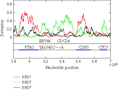
The reading-frame-specific PFDⁱ, i = 1,2,3 curves for a segment of DNA in yeast chromosome I (from nucleotide 58 000 to nucleotide 70 000). The sliding window size is w = 512. A 5th-order moving average filter has been applied. Colored horizontal bars on the two lines below the deviation curves are the open reading frames on the two strands of the chromosome, (first line: positive strand; second line: reverse strand). The orange and blue bars represent verified ORFs while a gray bar represents a dubious ORF.

Figure 6.

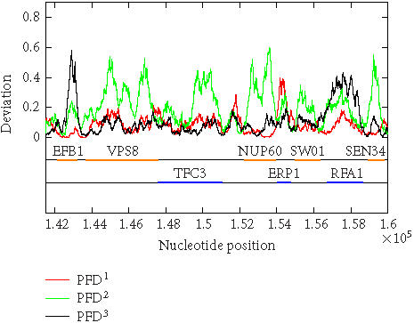
Period-3 fractal deviations (PFDs) of yeast chromosome I (a segment from nucleotide 141 500 to nucleotide 160 000).

We now evaluate the efficiency of the MAXFD as a codon index by studying all of the 16 yeast chromosomes. Our sample pool is comprised of two sets of DNA segments: the coding set, which contains 4125 verified ORFs (fully coding regions or exons), and the noncoding set, which contains 5993 segments (fully noncoding regions or introns). Different subsets of coding/noncoding segments are extracted according to the lengths of the sequence segments. These subsets are described by four parameters, N₁, n₁, N₂, n₂, where N₁ and N₂ are the numbers of coding and noncoding sequences with length greater than n₁ and n₂, respectively. After subsets of coding/noncoding sequences are chosen, MAXFD is then computed for all segments in those subsets. We denote the cumulative distribution of MAXFD over the two subsets as P_C(δ) and P_NC(δ). Then 1 − P_C(δ) is the proportion of coding segments in C with MAXFD > δ and P_NC(δ) is the proportion of noncoding segments in NC with MAXFD < δ. We define sensitivity as the proportion of segments in set C correctly labeled as “coding“ and specificity as the proportion of segments in set NC correctly labeled as “noncoding.” Given a threshold δ₀, the sensitivity and specificity are 1 − P_C(δ₀) and P_NC(δ₀), respectively. If we define the percentage accuracy as the average of sensitivity and specificity, an optimal decision threshold is often set at where sensitivity equals specificity. By plotting 1 − P_C(f) and P_NC(f) together, the optimal decision threshold is the abscissa of the point where the two curves intersect. The corresponding percentage accuracy is then simply 1 − P_C(δ₀) (or P_NC(δ₀), since P_NC(δ₀) = 1 − P_C(δ₀)). Figure 4 shows the sensitivity/specificity curves for four configurations of (n₁, n₂). More detailed statistics for all five configurations of (n₁, n₂) studied are summarized in Table 1, for two window sizes, w = 512 and 128. With sliding window size w = 512, the percentage accuracy on the entire sample pool is 82.5%. When only those segments longer than the window size are concerned, the accuracy is increased to 89.8%. For coding and noncoding subsets with segment lengths greater than 1026, the accuracy is further improved to 95.4%. While one might think the statistics shown in Table 1 may become a lot worse when a much smaller sliding window size is used, this is not the case. In fact, when the sliding window size is reduced to 128, the accuracy for the long coding/noncoding sequences is only slightly degraded, while the accuracy for the entire coding/noncoding sequences is actually improved. Overall, we would conclude that the codon index proposed is fairly independent of the sliding window size.

Table 1.

Accuracy of the PFD-based coding-region identification algorithm on different coding/noncoding subsets. The parameters N₁ and N₂ are the numbers of coding and noncoding sequences with length greater than n₁ and n₂, respectively. A DNA segment is declared “coding” if MAXFD > δ₀ and “noncoding” otherwise. Accuracy is defined as the average of sensitivity and specificity. The threshold δ₀ is set at where sensitivity equals specificity.

n1	N1	n2	N2	δ0	Sensitivity/specificity
					w = 512	w = 128
1	4125	1	5993	0.1800	82.5%	84.7%
256	4067	256	4186	0.1660	85.7%	86.7%
512	3756	512	1948	0.1500	89.8%	89.4%
1026	2674	512	1948	0.1620	92.5%	91.2%
1026	2674	1026	650	0.1320	95.4%	94.4%

In experiments involving expressed sequence tags (ESTs), the sequences available may all be short. Can the MAXFD index proposed still be useful? The answer is yes. When a sequence is very short, it is not necessary to use a sliding window to obtain three deviation curves. Instead one can simply obtain three values, PFD¹, PFD², PFD³, from the sequence and find MAXFD using (8). If the value is very large, one has good reason to assume that the suspected EST indeed belongs to a coding region. Otherwise, it may not. When the former is the case, the reading frame with the largest PFDⁱ, where i ∈ {1, 2, 3}, very likely indicates the correct reading frame (assuming there is no error in the sequence). When the sequence under study is not too short, one can then employ the sliding window technique. The PFD¹(m), PFD²(m), PFD³(m) curves that can be obtained this way will look like those obtained for a short segment of those shown in Figures 5 and 6. We note that the procedures outlined in this here have been applied to some experimentally obtained short DNA segments provided by Drs. Farmerie and Liu of the Institute of Biotechnology at the University of Florida.

References

- 1.Bennetzen J.L, Hall B.D. Codon selection in yeast. J Biol Chem. 1982;257(6):3026–3031. [PubMed] [Google Scholar]
- 2.Sharp P.M, Li W.H. The codon adaptation index—a measure of directional synonymous codon usage bias, and its potential applications. Nucleic Acids Res. 1987;15(3):1281–1295. doi: 10.1093/nar/15.3.1281. [DOI] [PMC free article] [PubMed] [Google Scholar]
- 3.Jansen R, Bussemaker H.J, Gerstein M. Revisiting the codon adaptation index from a whole-genome perspective: analyzing the relationship between gene expression and codon occurrence in yeast using a variety of models. Nucleic Acids Res. 2003;31(8):2242–2251. doi: 10.1093/nar/gkg306. [DOI] [PMC free article] [PubMed] [Google Scholar]
- 4.Zhang C.T, Wang J. Recognition of protein coding genes in the yeast genome at better than 95% accuracy based on the Z curve. Nucleic Acids Res. 2000;28(14):2804–2814. doi: 10.1093/nar/28.14.2804. [DOI] [PMC free article] [PubMed] [Google Scholar]
- 5.Staden R, McLachlan A.D. Codon preference and its use in identifying protein coding regions in long DNA sequences. Nucleic Acids Res. 1982;10(1):141–156. doi: 10.1093/nar/10.1.141. [DOI] [PMC free article] [PubMed] [Google Scholar]
- 6.Claverie J.M, Bougueleret L. Heuristic informational analysis of sequences. Nucleic Acids Res. 1986;14(1):179–196. doi: 10.1093/nar/14.1.179. [DOI] [PMC free article] [PubMed] [Google Scholar]
- 7.Farber R, Lapedes A, Sirotkin K. Determination of eukaryotic protein coding regions using neural networks and information theory. J Mol Biol. 1992;226(2):471–479. doi: 10.1016/0022-2836(92)90961-i. [DOI] [PubMed] [Google Scholar]
- 8.Fickett J.W, Tung C.S. Assessment of protein coding measures. Nucleic Acids Res. 1992;20(24):6441–6450. doi: 10.1093/nar/20.24.6441. [DOI] [PMC free article] [PubMed] [Google Scholar]
- 9.Fickett J.W. Recognition of protein coding regions in DNA sequences. Nucleic Acids Res. 1982;10(17):5303–5318. doi: 10.1093/nar/10.17.5303. [DOI] [PMC free article] [PubMed] [Google Scholar]
- 10.Shulman M.J, Steinberg C.M, Westmoreland N. The coding function of nucleotide sequences can be discerned by statistical analysis. J Theor Biol. 1981;88(3):409–420. doi: 10.1016/0022-5193(81)90274-5. [DOI] [PubMed] [Google Scholar]
- 11.Borodovsky M, Koonin E.V, Rudd K.E. New genes in old sequence: a strategy for finding genes in the bacterial genome. Trends Biochem Sci. 1994;19(8):309–313. doi: 10.1016/0968-0004(94)90067-1. [DOI] [PubMed] [Google Scholar]
- 12.Almagor H. Nucleotide distribution and the recognition of coding regions in DNA sequences: an information theory approach. J Theor Biol. 1985;117(1):127–136. doi: 10.1016/s0022-5193(85)80168-5. [DOI] [PubMed] [Google Scholar]
- 13.Silverman B.D, Linsker R. A measure of DNA periodicity. J Theor Biol. 1986;118(3):295–300. doi: 10.1016/s0022-5193(86)80060-1. [DOI] [PubMed] [Google Scholar]
- 14.Chechetkin V.R, Turygin A.Y. Size-dependence of 3-periodicity and long-range correlations in DNA sequences. Physics Lett A. 1995;199(1-2):75–80. [Google Scholar]
- 15.Tiwari S, Ramachandran S, Bhattacharya A, Bhattacharya S, Ramaswamy R. Prediction of probable genes by Fourier analysis of genomic sequences. Comput Appl Biosci. 1997;13(3):263–270. doi: 10.1093/bioinformatics/13.3.263. [DOI] [PubMed] [Google Scholar]
- 16.Trifonov E.N. 3-, 10.5-, 200- and 400-base periodicities in genome sequences. Physica A. 1998;249:511–516. [Google Scholar]
- 17.Yan M, Lin Z.S, Zhang C.T. A new Fourier transform approach for protein coding measure based on the format of the Z curve. Bioinformatics. 1998;14:685–690. doi: 10.1093/bioinformatics/14.8.685. [DOI] [PubMed] [Google Scholar]
- 18.Anastassiou D. Frequency-domain analysis of biomolecular sequences. Bioinformatics. 2000;16(12):1073–1081. doi: 10.1093/bioinformatics/16.12.1073. [DOI] [PubMed] [Google Scholar]
- 19.Issac B, Singh H, Kaur H, Raghava G.P. Locating probable genes using Fourier transform approach. Bioinformatics. 2002;18(1):196–197. doi: 10.1093/bioinformatics/18.1.196. [DOI] [PubMed] [Google Scholar]
- 20.Kotlar D, Lavner Y. Gene prediction by spectral rotation measure: a new method for identifying protein-coding regions. Genome Res. 2003;13(8):1930–1937. doi: 10.1101/gr.1261703. [DOI] [PMC free article] [PubMed] [Google Scholar]
- 21.Li W, Kaneko K. Long-range correlation and partial 1/fa spectrum in a non-coding DNA sequence. Europhys Lett. 1992;17(7):655–660. [Google Scholar]
- 22.Peng C.K, Buldyrev S.V, Goldberger A.L, et al. Long-range correlations in nucleotide sequences. Nature. 1992;356(6365):168–170. doi: 10.1038/356168a0. [DOI] [PubMed] [Google Scholar]
- 23.Voss R.F. Evolution of long-range fractal correlations and 1/f noise in DNA base sequences. Phys Rev Lett. 1992;68(25):3805–3808. doi: 10.1103/PhysRevLett.68.3805. [DOI] [PubMed] [Google Scholar]
- 24.Mandelbrot B.B. The Fractal Geometry of Nature. New York, NY: W. H. Freeman; 1982. [Google Scholar]
- 25.Azbel M.Y. Random two-component one-dimensional Ising model for heteropolymer melting. Phys Rev Lett. 1973;31:589–592. [Google Scholar]
- 26.Zhang C.T, Zhang R, Ou H.Y. The Z curve database: a graphic representation of genome sequences. Bioinformatics. 2003;19(5):593–599. doi: 10.1093/bioinformatics/btg041. [DOI] [PubMed] [Google Scholar]
- 27.Berthelsen C.L, Glazier J.A, Skolnick M.H. Global fractal dimension of human DNA sequences treated as pseudorandom walks. Phys Rev A. 1992;45(12):8902–8913. doi: 10.1103/physreva.45.8902. [DOI] [PubMed] [Google Scholar]
- 28.Cebrat S, Dudek M.R, Gierlik A, Kowalczuk M, Mackiewicz P. Effect of replication on the third base of codons. Physica A. 1999;265(1-2):78–84. [Google Scholar]
- 29.Stanley H.E, Buldyrev S.V, Goldberger A.L, Havlin S, Peng C.K, Simons M. Scaling features of noncoding DNA. Physica A. 1999;273(1-2):1–18. doi: 10.1016/s0378-4371(99)00407-0. [DOI] [PubMed] [Google Scholar]
- 30.Karlin S, Brendel V. Patchiness and correlations in DNA sequences. Science. 1993;259(5095):677–680. doi: 10.1126/science.8430316. [DOI] [PubMed] [Google Scholar]
- 31.Peng C.K, Buldyrev S.V, Havlin S, Simons M, Stanley H.E, Goldberger A.L. Mosaic organization of DNA nucleotides. Phys Rev E Stat Phys Plasmas Fluids Relat Interdiscip Topics. 1994;49(2):1685–1689. doi: 10.1103/physreve.49.1685. [DOI] [PubMed] [Google Scholar]
- 32.Viswanathan G.M, Buldyrev S.V, Havlin S, Stanley H.E. Long-range correlation measures for quantifying patchiness: Deviations from uniform power-law scaling in genomic DNA. Physica A. 1998;249(1-4):581–586. [Google Scholar]
- 33.Ossadnik S.M, Buldyrev S.V, Goldberger A.L, et al. Correlation approach to identify coding regions in DNA sequences. Biophys J. 1994;67(1):64–70. doi: 10.1016/S0006-3495(94)80455-2. [DOI] [PMC free article] [PubMed] [Google Scholar]