Reliable estimation via hybrid gradient boosting machine for mud loss volume in drilling operations

Abstract

Mud loss during drilling operations poses a significant problem in the oil and gas industry due to its contributions to increased costs and operational risks. This study aims to develop a reliable predictive model for mud loss volume using machine learning techniques to improve drilling efficiency and reduce non-productive time. The dataset consists of 949 field records from Middle Eastern drilling sites, incorporating variables such as borehole diameter, drilling fluid viscosity, mud weight, solid content, and pressure differential. Initial data analysis included statistical evaluation, outlier detection using leverage diagnostics, and data normalization to ensure validity and consistency. A Gradient Boosting Machine (GBM) served as the core predictor, with its hyperparameters fine-tuned using four optimization strategies: Evolution Strategies (ES), Batch Bayesian Optimization (BBO), Bayesian Probability Improvement (BBI), and Gaussian Process Optimization (GPO). Model performance was evaluated using k-fold cross-validation, with metrics including R², mean squared error and average absolute relative error percentage. Results demonstrated that the GBM-BPI achieved the strongest test performance (R² = 0.926, MSE = 1208.77, AARE% = 26.73), outperforming other approaches in accuracy and stability. Feature importance assessed through SHAP analysis revealed that hole size, formation type, and pressure differential were the most influential variables, while solid content had minimal effect.

Introduction

Mud loss, commonly called lost circulation, is a longstanding and critical challenge in drilling operations worldwide, resulting in higher operational costs, prolonged non-productive time, and increased safety and environmental risks^1–3. The problem is especially prevalent in reservoirs with complex geo-mechanical conditions and areas with exceptionally narrow operational mud-weight windows. In these scenarios, the balance between the pressure exerted by the drilling fluid and the formation strength is delicate; even minor deviations can result in the unintended loss of drilling fluid into the surrounding formation. Regions with extensive carbonate reservoirs, such as those found in the Middle East, are particularly susceptible due to the development of loss zones in fractured, vuggy, or highly permeable formations^3–7.

Various operational factors influence mud loss during drilling. The most significant are borehole geometry, drilling fluid viscosity, solid content, mud weight, and the pressure differential between the wellbore and the formation. These variables interact with formation properties, including permeability and fracture characteristics, to determine the likelihood and severity of fluid loss events^8–11. Maintaining the so-called ‘mud window,’ defined by pore pressure and fracture gradient, is essential for preserving wellbore integrity. Deviations from this operational window can quickly lead to incidents of mud loss or even catastrophic formation failure^12–14.

Historically, conventional strategies to address mud loss problems include preventive and remedial measures. Preventive approaches focus on optimizing the composition and properties of drilling fluids and using specialized materials designed to strengthen the wellbore. Remedial techniques often involve adding lost circulation materials into the drilling fluid to bridge or seal fractures^15–17. However, the success of these interventions is hampered by a limited understanding of subsurface fracture widths and the dynamic behavior of fluids under high-pressure and high-temperature conditions. Many decisions regarding lost circulation treatments rely heavily on field experience and trial and error^18–20.

Analytical and numerical models have been developed to predict fluid loss rates and inform drilling practices, but these frameworks face substantial challenges in accounting for the complex interplay of geological and operational factors. Models often require extensive calibration and may not generalize well across different fields or well types. The ability to obtain accurate predictions is further hampered by the variability and limitations of traditional monitoring systems, such as paddle flowmeters or pit volume totalizer systems, which provide only intermittent and sometimes imprecise measurements of fluid levels and loss rates^21–23.

Recent advancements in sensor technology have allowed for improved data collection, yet real-time, high-resolution data on mud loss events remain scarce. The complexity of downhole environments, varying operational parameters, and difficulty measuring certain formation and drilling fluid characteristics increase the uncertainty involved in traditional prediction and detection methods^24–26. Amid these challenges, artificial intelligence and machine learning have emerged as promising tools for prediction and control in various disciplines^27–30. Machine learning algorithms, particularly those designed to handle large, multi-dimensional datasets, offer superior capacity to model non-linear relationships between drilling parameters and mud loss outcomes. Approaches such as artificial neural networks, support vector machines, random forests, and gradient boosting machines have been successfully applied to various tasks, including identifying lost circulation risk zones, estimating mud loss rates, and optimizing lost circulation materials. These models leverage historical and real-time data to identify complex patterns that are often unrecognizable through traditional analytical approaches^23,24,31. For example, Alkouh et al.³² presented an artificial neural network (ANN) model to predict plastic viscosity of oil-based muds under high-pressure, high-temperature downhole conditions. It improved over traditional methods by offering an explicit, low-computation model validated on both training and unseen datasets. Pressure was found to be the dominant influencing factor. The model enabled real-time field predictions, reducing reliance on lab measurements. Agwu et al.³³ introduced a novel application of Multivariate Adaptive Regression Splines (MARS) to model mud viscosity at downhole conditions using temperature, pressure, and surface viscosity. The MARS model offered better interpretability and flexibility than ANN and traditional regression, though with moderate accuracy. It provided the first documented use of MARS in drilling mud modeling, especially for both oil- and water-based muds. Agwu et al.³⁴ provided a highly accurate ANN model to predict CO₂ solubility in 20 types of ionic liquids across a wide range of temperatures and pressures. The model was explicitly formulated, computationally efficient, and interpretable via connection weight analysis. This tool could aid solvent selection for carbon capture in gas processing industries, improving efficiency and reducing equipment corrosion. Atefi et al.³⁵ using Bayesian regularized ANN, predicted CO₂ diffusivity in heavy crude oils and bitumen for EOR applications. The model was explicit, accurate (R² = 0.996), fast, and validated for generalizability. Sensitivity analysis shows pressure and temperature as dominant variables, and the work emphasized ease of industrial use and physical interpretability. Atefi et al. also³⁶ developed machine learning models (CNN, ELM, LSTM) for estimating the heat capacity of deep eutectic solvents using 2,696 data points. CNN showed the best performance, and SHAP analysis provided insights into feature importance. The model reduces experimental needs, ensures physical consistency, and supports DES formulation and selection in green chemistry and industrial processes.

Integrating evolutionary algorithms for hyperparameter optimization in machine learning models has improved predictive performance and robustness. Hybrid models combining advanced ensemble learning techniques with systematic optimization strategies have outperformed conventional models, offering rapid convergence and better generalizability for challenging, non-linear drilling problems. Additionally, recent developments in interpretability tools, such as SHapley Additive exPlanations (SHAP), now allow for transparent quantification of feature influence, helping engineers understand which inputs most significantly impact mud loss predictions^37–39.

While advances have been made in machine learning for drilling operations, most studies focus on simply classifying whether mud losses will occur rather than accurately predicting the volume of mud lost with high resolution or utilizing real-time field data. This restricts practical impact in operational settings. The research highlighted here addresses this gap by developing an interpretable ML model to accurately forecast mud loss, which is vital in preventing costly and hazardous drilling incidents. The workflow begins with robust empirical data collection and comprehensive preprocessing, including outlier detection and normalization. A Gradient Boosting Machine model is then built and rigorously validated using k-fold cross-validation, with its hyperparameters optimized through several algorithms (ES, BBO, BPI, and GPO). Model evaluation combines statistical metrics and SHAP-based feature analysis, enhancing interpretability and ensuring key variables influencing mud loss are clearly understood, thereby improving decision-making and model transparency. Figure 1 illustrates the overall workflow of this study.

Fig. 1.

The overall workflow of mud loss prediction implemented in this study.

Data gathering and analysis

Statistical analysis of the dataset

The dataset employed in this study for developing and validating the predictive model was derived from empirical field measurements on mud loss volumes recorded during drilling operations in the Middle East. In this dataset, the response variable is the volume of mud loss. In contrast, the predictor variables include borehole diameter (inches), drilling fluid viscosity (centipoise, cp.), solid content (percentage), and the pressure differential between the drilling fluid and the reservoir (pounds per square inch, psi).

A total of 949 data entries comprise this dataset. For model construction, 90% of these records were allocated to the training set, and the remaining 10% were reserved for model testing. This task was conducted randomly. The distribution and range of each variable in the dataset are depicted by violin plots in Fig. 2.

Fig. 2.

Violin plots illustrating the distributions of input and output variables used in this research.

This section examines the influence of each input feature on the target variable (mud loss volume). The study quantifies the significance and contribution of each predictor using a relevance coefficient calculated according to the following Eqs.^40,41:

1

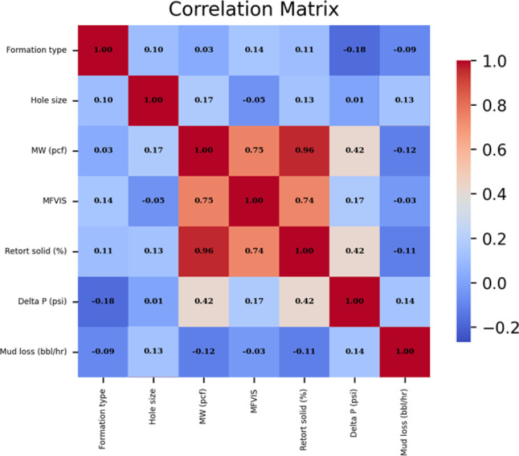
where j denotes the specific predictor under evaluation, the relevance coefficient ranges between − 1 and + 1, with values approaching + 1 indicating a strong positive association between an input and the output and values near − 1 signifying a strong negative association. A positive coefficient means that increases in the predictor variable lead to higher mud loss, while a negative coefficient suggests an inverse effect. As illustrated in Fig. 3, larger hole sizes and greater pressure differential are associated with increased mud loss, as evidenced by their positive relevance coefficients. In contrast, parameters such as drilling fluid viscosity, mud weight, and solid content demonstrate negative correlations, indicating their potential to reduce mud loss volume during drilling operations.

Fig. 3.

Relevance coefficients of input variables used to assess their influence on mud loss volume in drilling operations.

Before applying machine learning algorithms and model development, leverage diagnostics were employed to assess the presence of outliers and influential observations within the dataset⁴². Figure 4 presents the distribution of Hat values computed for each data point, utilizing leverage-based methodology for outlier detection.

Fig. 4.

Hat value distribution for all data points using leverage analysis for outlier detection.

Each point corresponds to a data sample in this graphical representation, and its Hat value reflects its relative influence on the overall regression model. Observations with unusually high Hat values are considered potential outliers or influential points that may disproportionately affect model training and prediction outcomes. As illustrated in Fig. 4, only approximately 1% of the data points exhibit Hat values greater than 0.02, which is commonly regarded as a threshold for identifying unusually influential samples. Most data points fall within the acceptable range, indicating a uniform influence across the dataset. These findings affirm the overall integrity and validity of the dataset, suggesting that it is largely free from strongly influential outliers that could compromise the robustness or generalizability of subsequent machine learning models. As a result, the dataset is suitable for reliable model development and evaluation. Notice that we considered all the data within the process of model development in order to make them as highly generalized as possible.

Gradient boosting and optimization algorithms background

Gradient boosting machine

GBM is a supervised learning methodology broadly applicable to regression and classification tasks. As an ensemble learning technique, GBM constructs a predictive model by sequentially combining multiple weak learners, typically decision trees, to achieve high predictive performance. This sequential integration is achieved by iteratively minimizing a specified loss function, which quantifies the error between predicted outputs and actual target values through gradient descent.

The core concept of GBM involves sequentially improving the modeling accuracy by correcting the errors of previous learners, thereby building a more robust ensemble model. Given a dataset consisting of n observations with input features xi​ and their corresponding target values yi​, the objective is to approximate the underlying function F(x) such that F(x) closely matches y.

The algorithm commences with constructing a simple initial model, often chosen as a constant that minimizes the selected loss function across the dataset. For instance, in regression tasks employing the mean squared error loss, the optimal initial prediction is the mean of the target variable. Mathematically, the initial model can be expressed as:

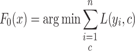2

where L represents the loss function, and c is a constant value. After establishing the initial model, GBM proceeds stage-wise by introducing new weak learners in each iteration. At the n-th iteration, a new learner h_m​(x) is trained to fit the loss function’s negative gradient (residuals) concerning the current ensemble prediction. The model update at each step is defined as follows:

3

In this equation, F_m−1​(x) is the model from the previous iteration, h_m​(x) is the new weak learner, and η is the learning rate that controls the contribution of each new learner to the whole ensemble.

Several hyperparameters significantly influence the performance and behavior of GBM. The number of boosting iterations, denoted as M, determines how many weak learners are incorporated into the model. Increasing M can enhance model accuracy on training data but also increase the overfitting risk. The learning rate η is a scaling parameter that adjusts the influence of each added learner; smaller values of η require more iterations but can improve model generalization. The maximum depth of decision trees restricts model complexity and helps prevent overfitting, while other regularization strategies, such as specifying a minimum number of samples required at split nodes, further enhance model robustness.

GBM offers notable flexibility by allowing the use of arbitrary differentiable loss functions, adapting readily to regression, binary classification, and multiclass classification tasks. Additional techniques, such as stochastic gradient boosting, employ random subsampling of the data at each iteration to improve computational efficiency and reduce variance.

Despite its advantages, GBM faces certain challenges. The algorithm is sensitive to hyperparameter tuning, and overfitting may occur if the model grows too complex or if an excessive number of learners is used. The sequential nature of gradient boosting can also lead to significant computational demand, particularly with large datasets.

GBM has found widespread application in industries such as finance for credit risk assessment and fraud detection, healthcare for predicting clinical outcomes, and e-commerce for recommendation systems. Specialized implementations such as XGBoost, LightGBM, and CatBoost have been developed to address efficiency and scalability concerns. These libraries offer enhanced performance, advanced handling of different data types, and support for large-scale distributed training^43–45.

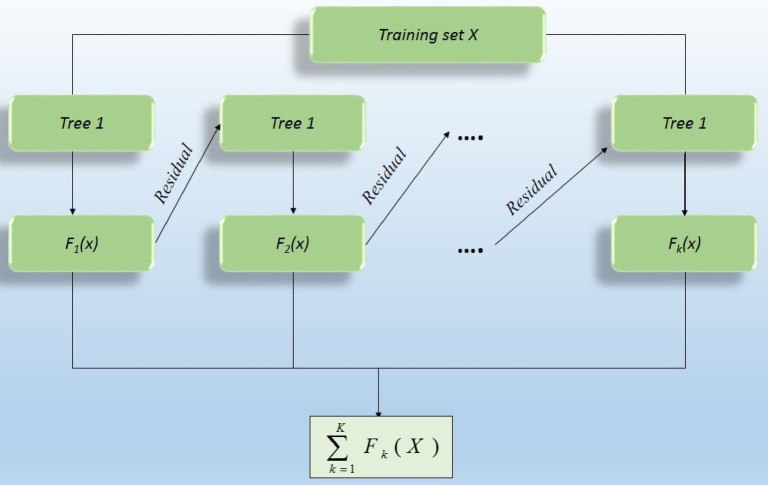
In summary, Gradient Boosting Machines are a fundamental element of modern machine learning, providing resilient solutions for complex modeling challenges. Integrating multiple weak learners through gradient-based optimization and the capacity to address various predictive tasks have established GBM as a highly effective tool for practical applications and academic research. Figure 5 displays a flowchart summarizing the main steps of the Gradient Boosting Machine algorithm.

Fig. 5.

Flowchart (left) and structural schematic representation of gradient boosting algorithm.

Optimization algorithms

This section briefly discusses the metaheuristic optimization algorithms used in the study.

Gaussian process optimization (GPO)

Gaussian Process Optimization (GPO) is a probabilistic methodology designed to optimize objective functions that are costly or time-consuming to evaluate. At the core of this approach lies the use of Gaussian Processes (GPs) to construct a surrogate model, which efficiently approximates the true objective function. A Gaussian Process is fully characterized by a mean function m(x) and a covariance function or kernel k(x, x′), ensuring that any finite collection of function values follows a joint Gaussian distribution.

4

This surrogate model provides predictions of the objective function values at unobserved points and quantifies the associated uncertainty. This dual capability enables GPO to strategically balance exploration sampling where the surrogate predicts favorable objective values. As new function evaluations are collected, the Gaussian Process surrogate is updated, iteratively refining its approximation of the objective function and guiding subsequent sampling decisions.

A central component of GPO is using acquisition functions, which determine the next location in the input space to sample the objective function. Popular acquisition functions include Expected Improvement (EI), Probability of Improvement (PI), and Upper Confidence Bound (UCB). For example, the EI acquisition function prioritizes regions with the greatest expected gain over the current best value, while UCB offers a tunable mechanism to balance exploration and exploitation via a confidence parameter. The acquisition function effectively directs sampling toward areas of the search space likely to yield improvements or where information about the objective function is insufficient. This approach is particularly advantageous when objective function evaluations are expensive, noisy, or limited in number.

5

The GPO process typically unfolds iteratively. Initially, a small set of observations is gathered to fit the Gaussian Process model. The surrogate model evaluates the acquisition function in each subsequent iteration to identify promising sampling locations. The surrogate model is updated with the new data after evaluating the objective function at the chosen points. This cycle continues until a predefined stopping condition is reached, such as a computational budget limit or convergence of the optimization metric. GPO is especially suitable for high-cost optimization scenarios because of its iterative and data-efficient approach.

The versatility of GPO has led to its widespread adoption across various domains. It is commonly used for hyperparameter tuning in machine learning, engineering design optimization, and experiment planning in the physical sciences. The framework’s capacity to explicitly model uncertainty and make efficient sampling decisions under data or evaluation constraints has established GPO as a premier tool for optimization tasks where function evaluations are particularly resource-intensive^46,47.

Evolutionary strategies

ES is a class of stochastic, population-based optimization algorithms inspired by the principles of natural evolution. These methods are particularly effective for solving continuous optimization problems, where the search space is often complex and high-dimensional. In ES, a population of potential solutions undergoes iterative improvement across generations, driven by evolutionary operations such as mutation, recombination, and selection.

Each individual within the population is modeled as a pair (x,σ), where x denotes the solution vector, and σ represents a corresponding vector of strategy parameters. The strategy parameters control the magnitude of mutation applied to each dimension of x, thereby influencing the exploration capabilities of the algorithm⁴⁸.

The ES procedure begins with the initialization of a population comprising µ individuals. The initial solution vectors x are typically sampled randomly within the defined bounds of the search space, whereas the strategy parameters σ are assigned small, positive values. Formally, this can be expressed as:

6

where x^min and x^max​ specify the permissible range for each x component, and σ^min and σ^max ​ define the range for σ.

During each generation, λ offspring are generated through mutation, wherein the solution vectors and their respective strategy parameters are perturbed according to defined stochastic rules. The updated strategy parameters, denoted as σ_i′​, are typically calculated by:

7

N(0,1) and Ni​(0,1) represent standard normal random variables in this equation. The coefficients τ and τ′ are learning rates conventionally determined by the problem’s dimensionality⁴⁴. The solution vector is subsequently updated as follows:⁴⁹:

8

Recombination, when employed, constructs offspring by combining information from multiple parent individuals. For intermediate recombination, the new solution and strategy parameters are produced as weighted averages of the parents:

9

10

Following offspring generation, the selection phase determines which individuals constitute the next generation. In the (µ + λ)-ES scheme, the top µ individuals are chosen from the combined set of parents and offspring, whereas in the (µ,λ)-ES strategy, selection is performed exclusively among the offspring, with λ ≥ µ. Both approaches encourage steady progress towards improved solutions over successive generations.

A significant advantage of Evolution Strategies lies in their self-adaptive mechanism, which autonomously adjusts the strategy parameters σ as the search proceeds. This capability facilitates a dynamic equilibrium between exploring the broader parameter space and exploiting promising regions, making ES robust in addressing complex and high-dimensional optimization tasks. Further extensions, such as the Covariance Matrix Adaptation Evolution Strategy (CMA-ES), improve performance by adapting the covariance structure of the mutation distribution.

In summary, Evolution Strategies systematically develop and refine a population of candidate solutions using iterative mutation, recombination, and selection application. The self-adaptation of strategy parameters enhances the algorithm’s adaptability and resilience, particularly for ongoing and challenging optimization problems. The ES workflow incorporates population initialization, offspring production via mutation and recombination, fitness evaluation, selection of the best individuals, and repetition until a predefined stopping criterion is met. The iterative process yields an optimal solution as its final output⁵⁰.

Bayesian probability improvement (BPI)

BPI is a specialized acquisition function commonly employed within the Bayesian optimization framework, especially when optimizing expensive black-box functions. Bayesian optimization provides an effective strategy for global optimization in scenarios where evaluating the objective function is computationally demanding, as it aims to identify optimal solutions while minimizing the number of function evaluations required. Within this context, BPI guides the search process by systematically balancing exploring uncertain areas with exploiting regions that are likely to yield favorable outcomes.

The principal objective of the BPI acquisition function is to maximize the probability that a newly selected candidate point will yield an objective function value surpassing the best observation to date. Unlike alternative acquisition functions such as Expected Improvement (EI) or Upper Confidence Bound (UCB), BPI distinctly quantifies the probability of improvement rather than focusing on the expected magnitude or the trade-off between mean and uncertainty. This characteristic makes BPI particularly valuable in applications where it is critical to increase the likelihood of identifying superior solutions rather than merely optimizing the expected gain.

BPI estimates the probability that the objective function value at a candidate point x will exceed the current best value, denoted f(x⁺). This probability is computed using the posterior mean µ(x) and variance σ²(x) obtained from a Gaussian Process (GP) model, which serves as a flexible probabilistic surrogate in Bayesian optimization. The probability of improvement at a point x is calculated via the cumulative distribution function (CDF) of the standard normal distribution as follows⁵¹.

The BPI is mathematically formulated as:

11

Here, Φ denotes the standard normal CDF, µ(x) is the predicted mean, σ(x) is the predictive standard deviation at x, and f(x⁺) represents the highest objective value obtained so far.

In practice, the BPI acquisition function prioritizes candidate points with the highest probability of improving over the best solution. Higher BPI values indicate a greater likelihood of surpassing the best-known outcome, thus steering the optimization process toward more probable solutions to yield advancement. This approach is particularly advantageous when consistent progress with each evaluation is desired, as it favors the probability of making improvements over the potential scale of such improvements.

In summary, the BPI acquisition function leverages the predictive uncertainty derived from a Gaussian Process model to navigate the search space in pursuit of optimal solutions efficiently. By emphasizing the probability of improvement, BPI is a valuable component within Bayesian optimization, especially in scenarios characterized by expensive or limited objective function evaluations and a need to increase the chances of discovering improved solutions⁵².

Batch bayesian optimization (BBO)

The Batch Bayesian Optimization (BBO) extends the standard Bayesian optimization (BO) framework by enabling the simultaneous evaluation of multiple candidate points, referred to as a “batch,” during each iteration. This approach is particularly advantageous in environments with parallel computing resources, such as high-performance computing clusters or distributed systems, where concurrent execution can be fully exploited. By leveraging parallelism, BBO significantly reduces the total wall-clock time required for optimization while retaining the robust global search characteristics inherent to Bayesian optimization.

The most notable advancement of BBO is its methodology for selecting a batch of points for evaluation, as opposed to the traditional sequential selection of individual candidates. This transition necessitates modifying the acquisition function to account for potential dependencies and correlations among the batch members since information gained from evaluating one candidate can inform the evaluations of others within the same batch.

Acquisition functions employed in BBO are adapted to maintain an effective balance between exploring uncertain regions and exploiting known promising areas across the batch. A widely adopted technique is the Parallel Expected Improvement (q-EI) acquisition function, which generalizes the traditional Expected Improvement (EI) criterion to a set of q points. The q-EI function estimates the collective expected improvement obtainable by simultaneously evaluating all points in the batch, considering the joint posterior distribution as modeled by a Gaussian Process (GP)⁵³. The formal definition of the q-EI function is expressed as⁵³:

12

where X= [x1​,x2​,…,xq​] denotes the batch of q points to be evaluated, f(X) represents their associated objective function values, f(x⁺) is the best objective value observed thus far, and E indicates the expectation concerning the joint posterior distribution of the GP at the batch points.

By incorporating the joint uncertainty and interdependencies among batch members, q-EI ensures that the selected candidate collection maximizes the expected improvement collectively, rather than treating each point in isolation. Other strategies, such as the extension of Thompson Sampling, have also been introduced to support effective batch selection under the Bayesian paradigm.

Overall, Batch Bayesian Optimization enhances the scalability and efficiency of conventional Bayesian optimization in computationally intensive scenarios. By exploiting parallel evaluation capabilities alongside specialized acquisition functions like q-EI, BBO effectively accelerates the optimization process without compromising the capacity to discover globally optimal solutions. Consequently, BBO is particularly well suited for contexts where rapid progress is required and parallel computing resources are available⁵⁴.

Modeling methodology

K-fold cross-validation is a robust statistical technique widely utilized for assessing the performance of machine learning models. The methodology involves partitioning the original training dataset into k equally sized subsets, referred to as “folds.” During each iteration, the model is trained on k − 1 folds and validated on the remaining fold, which serves as the temporary validation set. This process is repeated k times, with each fold being used exactly once as the validation set. By averaging the evaluation metrics across all k iterations, k-fold cross-validation provides a more dependable estimate of model performance, thereby reducing the risk of overfitting or underfitting that may arise with a single train–test split.

A key advantage of k-fold cross-validation lies in its efficient utilization of available data, making it particularly advantageous when working with limited datasets. The method ensures that every data instance participates in training and validation exactly once, minimizing biases associated with arbitrary train–test splits. This comprehensive approach supports fair model comparisons and facilitates effective hyperparameter tuning, ultimately contributing to a more objective evaluation of model generalizability. Furthermore, by systematically rotating the validation set, k-fold cross-validation mitigates the risk of overfitting, which is especially critical for small or moderately sized datasets.

The selection of the parameter k significantly influences both the computational cost and the reliability of the performance estimates. Conventional choices, such as k = 5 or k = 10, offer a practical trade-off between computational efficiency and the precision of the model evaluation. Smaller values of k may introduce higher variance in the results, while larger values, although providing more stable estimates, require proportionally greater computational effort. Variants such as stratified k-fold cross-validation further enhance the method by preserving class proportions within each fold, making it suitable for handling imbalanced datasets and preventing the underrepresentation of minority classes in any given fold^55,56.

In summary, k-fold cross-validation is a versatile and reliable approach for model evaluation and selection within machine learning pipelines. Its ability to yield unbiased and comprehensive assessments underpins its widespread adoption, particularly in contexts where rigorous model comparison and validation are essential. The overall structure of k-fold cross-validation is depicted in Fig. 6.

Fig. 6.

Schematic representation of the k-fold cross-validation process.

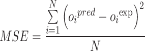
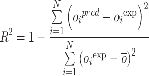
In this study, a 5-fold cross-validation approach is applied throughout the training and optimization of the random forest algorithm. Several evaluation metrics are employed to rigorously assess the predictive accuracy of the various hybrid models, including RE%, AARE%, MSE, and R², as defined below. Here, the subscript i denotes an individual data instance, while “pred” and “exp” represent the predicted and experimental (observed) values, respectively. The parameter N corresponds to the total number of data points^57–62:

13

14

15

16

The input features used for model development encompass hole size, mud weight, differential pressure, mud viscosity, and solid content. The target variable for prediction is the mud loss volume during drilling operations. Before model development, all input data are subjected to normalization:

17

In this context, n represents the original data value, while “min,” “max,” and “norm” correspond to the minimum value, maximum value, and the normalized value, respectively. This normalization procedure enhances the reliability of model evaluation by minimizing the effects of data variability and scale differences.

Results and discussion

Hyperparameter determination and optimization efficiency

Table 1 summarizes the optimal hyperparameters identified for Gradient Boosting Machine (GBM) models using four prominent optimization strategies: Evolution Strategies (ES), Batch Bayesian Optimization (BBO), Bayesian Probability Improvement (BPI), and Gaussian Process Optimization (GPO). The table indicates notable variations in the hyperparameter settings selected by each algorithm, underscoring the influence of the optimization method on model configuration.

Table 1.

Hyperparameter search space and optimal settings for GBM identified by four optimization algorithms.

Parameter	Range	ES	BBO	BPI	GPO
n_estimators	[50, 300]	268	274	232	283
max_depth	[5, 20]	16	11	12	16
max_features	[0.1, 1.0]	0.5370	0.5167	0.5526	0.9568
min_samples_split	[0.01, 0.5]	0.0553	0.0547	0.0617	0.0429
learning_rate	[0.01, 0.3]	0.1885	0.1541	0.2202	0.2712
subsample	[0.5, 1.0]	0.9765	0.9332	0.9541	0.6036
min_samples_leaf	[0.01, 0.5]	0.0209	0.0221	0.0199	0.0219

Specifically, the n_estimators parameter displays the widest range, with GPO selecting the highest value (283) and BPI the lowest (232), suggesting that GPO favors more estimators to enhance model complexity. Similarly, max_depth is maximized with ES and GPO (16), while BBO and BPI yield lower values, potentially reflecting a more conservative approach to model deepening. The max_features and min_samples_split values are consistently similar across ES, BBO, and BPI, but GPO opts for a considerably higher proportion of features (0.957) and a lower minimum split threshold (0.043), indicating a preference for utilizing more features and producing smaller splits in the trees. Though GPO selects a relatively higher rate, learning_rate values are generally within a comparable range, possibly facilitating faster model convergence. Subsample values approach the upper end of the range for ES, BBO, and BPI, which may contribute to increased robustness, while GPO adopts a noticeably lower value (0.604), reflecting a different sampling strategy. Additionally, min_samples_leaf is consistently small across all methods, supporting fine data partitioning.

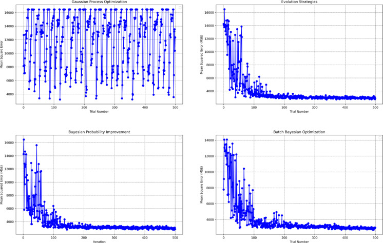
Figure 7 provides a dynamic comparison by plotting the Mean Squared Error (MSE) across iterative optimization steps for each algorithm. The results demonstrate that ES, BBO, and BPI achieve substantial reductions in MSE within the first 100 iterations, with their MSE values stabilizing and reaching minima as the optimization progresses to 500 iterations. This pattern highlights the efficient convergence and stability offered by these methods. In contrast, GPO exhibits persistent fluctuations in MSE throughout the iterations, suggesting possible challenges in attaining convergence or navigating a more complex error surface. These oscillations may be attributed to the inherent exploratory behavior of Gaussian Process-based optimization, which, while thorough in its search, might be more susceptible to local minima or sensitive to hyperparameter initializations.

Fig. 7.

MSE convergence curves across iterations for different GBM optimization algorithms.

Collectively, the findings in Table 1; Fig. 7 illustrate that while all optimization methods can effectively tune hyperparameters to improve GBM performance, ES, BBO, and BPI display superior convergence characteristics and stability compared to GPO in this experimental context. The observed differences highlight the importance of selecting an optimization strategy aligned with both computational efficiency and the specific characteristics of the dataset and learning task.

Figure 8 presents the total runtime, measured in seconds, for each GBM optimization algorithm. GPO demonstrates the fastest performance among the tested methods, completing the hyperparameter tuning process in 226 s. In comparison, BBO, BPI, and ES require 531, 572, and 605 s, respectively, indicating higher computational demands for these algorithms.

Fig. 8.

Comparison of total runtime in seconds for different GBM optimization algorithms.

Despite GPO’s advantage in computational speed, as illustrated by its minimal runtime, this efficiency does not translate to optimal model performance. Figure 7 shows that GPO experiences persistent instability in MSE convergence, undermining its suitability as a reliable optimization approach. In contrast, ES, BBO, and BPI each achieve more stable and effective MSE minimization, albeit at the cost of increased runtime. This highlights a critical trade-off: while GPO is computationally efficient, robust and consistent convergence—as exhibited by ES, BBO, and BPI—may warrant the additional computational investment for applications where prediction accuracy and model stability are prioritized.

Modeling evaluation

Table 2 compares the predictive performance of GBM models optimized by four different algorithms (GPO, ES, BPI, and BBO) across training and testing phases using R², MSE, and AARE% metrics. The results indicate that the GBM-BPI model achieves the highest predictive accuracy on the test set, as evidenced by the highest R² (0.926) and the lowest values for both mean squared error (MSE = 1208.768) and average absolute relative error percentage (AARE% = 26.727). This performance suggests that the Bayesian Probability Improvement (BPI) algorithm effectively balances model fit and generalization, outperforming the other tested approaches.

Table 2.

Performance metrics of GBM models optimized with different algorithms during training and test phases.

Optimization Algorithm	R2			MSE			AARE%
	Training	Test	Total	Training	Test	Total	Training	Test	Total
GBM-GPO	0.990	0.883	0.979	168.330	1904.603	342.140	10.354	38.495	13.171
GBM-ES	0.992	0.920	0.985	130.350	1306.443	248.083	8.303	28.980	10.373
GBM-BPI	0.991	0.926	0.985	145.053	1208.768	251.537	9.518	26.727	11.241
GBM-BBO	0.987	0.919	0.980	209.399	1317.484	320.324	11.824	29.061	13.549

Conversely, the model tuned with Gaussian Process Optimization (GBM-GPO) exhibits the lowest predictive capability on the test dataset, recording the lowest R² (0.883) and the highest error metrics among all algorithms examined. ES and BBO also yield competitive results, with ES closely following BPI regarding strong performance indicators on the test set.

Figure 9 offers a graphical representation of these evaluation metrics, visually highlighting the comparative differences in model accuracy and error rates across the four optimization strategies. Table 2; Fig. 9 confirm the robustness of the BPI algorithm in optimizing GBM for this application and underscore the importance of algorithm selection in achieving optimal predictive performance.

Fig. 9.

Visual comparison of GBM model performance metrics across various optimization algorithms.

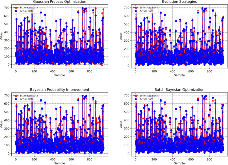
Figures 10 and 11, and 12 serve to comprehensively evaluate and contrast the predictive performance and error behavior of GBM models optimized via different algorithms.

Fig. 10.

Cross-plots of predicted versus actual values for GBM models optimized by different algorithms.

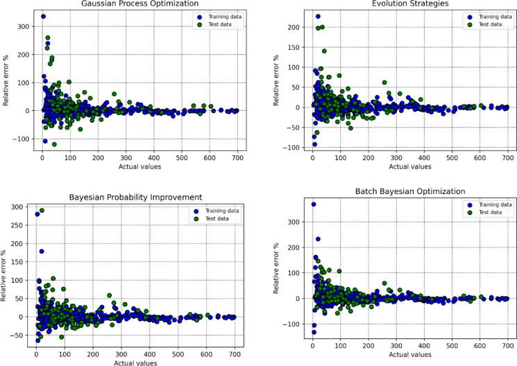
Fig. 11.

Relative error percentage (RE%) for each prediction across training and testing phases for the GBM models.

Fig. 12.

Comparison of actual and predicted values for GBM models optimized with various algorithms.

Figure 10 depicts cross-plots of predicted values against actual observations for training and testing datasets across all optimization algorithms. This form of visualization is instrumental in assessing the degree of concordance between predicted and real-world outcomes, facilitating direct interpretation of each model’s predictive calibration. Ideally, points should align closely with the y = x line, which denotes perfect prediction. The distribution and concentration of points relative to this line reveal critical information regarding systematic biases or under-/over-estimation tendencies within each optimization approach. Models exhibiting minimal scatter and strong alignment with the y = x line throughout both data subsets indicate superior generalization and predictive robustness, a key aspect in evaluating model validity.

Figure 11 presents the relative error percentage (RE%) for every prediction obtained during the training and testing. This granular error visualization allows for the in-depth inspection of prediction dispersion, highlighting the frequency and extremity of deviations across the full spectrum of data points. Models yielding RE% distributions highly concentrated around the y = 0 line, where prediction closely matches actual values, demonstrate accuracy and consistency in learning underlying data structures. Conversely, greater dispersion and larger outliers signify less reliable modeling, which may be attributable to the optimization algorithm’s overfitting, underfitting, or inherent limitations. Such detailed inspection of residual patterns can also help identify systematic errors or data regions prone to higher modeling uncertainty.

Figure 12 illustrates, for each instance, the magnitude of the difference between actual and predicted values derived from models tuned via various algorithms. This comparative trajectory analysis provides an intuitive visual cue regarding overall model fidelity: smaller, more consistent gaps correspond to superior alignment with empirical observations. This figure is particularly useful for visually tracking the stability and replicability of prediction performance across the dataset and identifying any localities where error magnitudes spike, potentially guiding further refinements or localized analysis.

Collectively, these visual analyses offer a multi-dimensional assessment that extends beyond aggregate statistical metrics, facilitating a deeper understanding of each algorithm’s strengths and limitations. Such comprehensive visual diagnostics are critical in discerning the overall predictive power of each approach and their error characteristics, reliability, and generalizability to unseen data. This integrative evaluation thus provides a robust foundation for selecting the most effective algorithmic framework for the GBM model in this problem context.

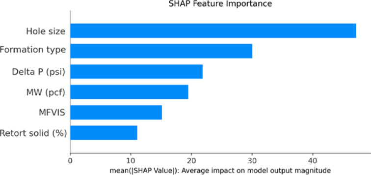
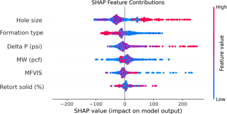
Figures 13 and 14 provide an interpretability analysis of the Random Forest model using SHAP (SHapley Additive exPlanations), an advanced technique for quantifying the contribution of each input feature to the model’s predictions. This approach, grounded in cooperative game theory, ensures a fair attribution of importance by considering all possible combinations of features and their marginal contributions to prediction outcomes^37,63,64.

Fig. 13.

Feature importance order determined through SHAP.

Fig. 14.

SHAP feature contributions graph.

Figure 13 displays the SHAP feature importance summary, where each bar reflects the average magnitude of the SHAP values for a given input variable. This quantitatively ranks feature influence on the predicted mud loss volume. The visualization reveals that ‘Hole Size’ exerts the largest impact on model outputs, emphasizing its critical role in the mud loss process. The subsequent features, such as ‘Formation Type’ and ‘Pressure Difference,’ also show substantial influence, reflecting their known physical or operational relevance in drilling contexts. By contrast, ‘Solid Content’ is shown to contribute minimally, which may indicate a lesser or more indirect relationship with mud loss within the observed data range.

Figure 14 presents the SHAP summary plot, which combines feature importance with the directionality of feature effects on individual predictions. Each point represents a single instance in the dataset, colored by the feature value (blue for low, red for high). The horizontal position indicates the SHAP value: positive values imply increased predicted mud loss, while negative values suggest a mitigating effect. Notably, high ‘Hole Size’ values (red points) cluster on the positive side of the SHAP axis, signaling that larger hole sizes drive higher mud loss predictions, a result consistent with drilling fluid dynamics theory, where increased borehole diameter can accelerate fluid loss due to larger exposed rock surfaces. Similarly, increased ‘Pressure Difference’ is associated with higher mud loss, as indicated by the aggregation of high-value, red points on the positive side. This trend aligns with established knowledge, as higher differential pressures promote greater fluid movement from the wellbore into the formation. Conversely, lower-importance features, such as ‘Solid Content,’ show less pronounced patterns, further supporting their weaker direct association with the target variable. The SHAP analysis reveals that hole size is the most influential factor in predicting mud loss rate during drilling, which aligns with literature indicating that larger boreholes increase the exposed formation area and reduce annular velocity, thereby elevating the risk of fluid invasion, especially in fractured or unconsolidated formations. Formation type is also critical, as lithologies like fractured carbonates or shales inherently possess higher loss susceptibility due to their pore structure and mechanical behavior. Pressure differential significantly contributes by driving fluid into formation fractures when wellbore pressure exceeds fracture gradient. Mud weight further influences hydrostatic pressure, where excessive values can fracture weak formations, escalating losses. Although less impactful, mud viscosity affects fluid rheology and filter cake quality, indirectly influencing loss control, while retort solids (%) play a minor role by altering equivalent circulating density, potentially increasing pressure but with limited direct effect on loss initiation.

In summary, the SHAP-based analyses in Figs. 13 and 14 identify primary influencers of mud loss predictions and elucidate the direction and nature of these relationships. These insights enhance model transparency and align with fundamental principles in drilling engineering, thereby supporting informed decision-making in real-world operations.

The findings of this study have significant implications for field development planning and drilling operations optimization. By identifying hole size, formation type, and pressure differential as the dominant contributors to mud loss, operators can implement targeted strategies such as optimizing borehole design, selecting appropriate mud weights, and customizing fluid systems based on lithological characteristics. The predictive model enables real-time decision-making during well planning, helping to mitigate risks of severe mud losses and reduce costly non-productive time. Incorporating this model into early-stage drilling design and monitoring workflows enhances operational efficiency, particularly in high-risk zones across Middle Eastern formations known for their variability in formation strength and permeability.

Despite its strong predictive performance, the model has certain limitations that warrant consideration. The dataset, while comprehensive, is region-specific, relying exclusively on 949 records from Middle Eastern drilling operations, which may limit generalizability to other geologies or operational contexts. Additionally, the model does not explicitly account for dynamic operational parameters such as real-time drilling rate, temperature variations, or fluid loss control additives, which could also influence mud loss behavior. The SHAP-based interpretability helps reveal feature importance but does not capture complex interactions between variables unless explicitly modeled, potentially oversimplifying some relationships inherent in the subsurface system. Future research should focus on expanding the dataset to include diverse geological settings and operational conditions to improve the model’s robustness and applicability across different drilling environments. Integrating real-time data streams, such as rate of penetration, annular pressure, and downhole temperature, can enhance predictive accuracy and enable dynamic loss control during drilling. Additionally, incorporating geomechanical models and reservoir simulation tools with machine learning can provide a more holistic view of formation behavior under stress. Comparative studies using deep learning architectures and hybrid modeling frameworks are also recommended to explore further gains in predictive performance and interpretability.

Conclusions

This study presents a comprehensive approach to predicting mud loss volume during drilling operations by applying advanced machine learning techniques. When optimized with Bayesian Probability Improvement, the Gradient Boosting Machine demonstrated the best overall predictive performance based on R², MSE, and AARE% metrics. The comparative evaluation showed that while all optimization algorithms tested enhanced model performance, stability, and predictive accuracy were highest with Bayesian Probability Improvement with R² = 0.926, MSE = 1208.77, AARE% = 26.73 for the testing stage. SHAP-based feature importance analysis indicated that borehole diameter and pressure differential impact mud loss prediction most, aligning with established engineering understandings of drilling processes. The systematic methodology encompassing rigorous data validation, model optimization, and interpretability provides a robust and transparent framework, supporting improved operational decisions to minimize mud loss and associated costs in drilling activities. Future research should focus on expanding the dataset to include diverse geological settings and operational conditions to improve the model’s robustness and applicability across different drilling environments.

Author contributions

All authors contributed equally to this research paper.

Data availability

Data supporting this study’s findings is made available from the corresponding upon plausible academic request.

Declarations

Competing interests

The authors declare no competing interests.

References

- 1.Nascimento, D. R. et al. Effects of particle-size distribution and solid additives in the apparent viscosity of drilling fluids. J. Petrol. Sci. Eng.182, 106275 (2019). [Google Scholar]
- 2.Borges, R. F. O. et al. Reparameterization of static filtration model of aqueous-based drilling fluids for simultaneous Estimation of compressible mudcake parameters. Powder Technol.386, 120–135 (2021). [Google Scholar]
- 3.Elkatatny, S., Mahmoud, M. & Nasr-El-Din, H. A. Filter cake properties of water-based drilling fluids under static and dynamic conditions using computed tomography scan. J. Energy Res. Technol.135 (4), 042201 (2013). [Google Scholar]
- 4.Bezemer, C. & Havenaar, I. Filtration behavior of Circulating drilling fluids. Soc. Petrol. Eng. J.6 (04), 292–298 (1966). [Google Scholar]
- 5.Yao, R. et al. Effect of water-based drilling fluid components on filter cake structure. Powder Technol.262, 51–61 (2014). [Google Scholar]
- 6.Sun, H. et al. Theoretical and numerical methods for predicting the structural stiffness of unbonded flexible riser for deep-sea mining under axial tension and internal pressure. Ocean Eng.310, 118672 (2024). [Google Scholar]
- 7.Yu, H. et al. Modeling thermal-induced Wellhead growth through the lifecycle of a well. Geoenergy Sci. Eng.241, 213098 (2024). [Google Scholar]
- 8.Bageri, B. S. et al. Effect of different weighting agents on drilling fluids and filter cake properties in sandstone formations. ACS Omega. 6 (24), 16176–16186 (2021). [DOI] [PMC free article] [PubMed] [Google Scholar]
- 9.Cheraghian, G. Nanoparticles in drilling fluid: A review of the state-of-the-art. J. Mater. Res. Technol.13, 737–753 (2021). [Google Scholar]
- 10.Ma, T., Peng, N. & Chen, P. Filter cake formation process by involving the influence of solid particle size distribution in drilling fluids. J. Nat. Gas Sci. Eng.79, 103350 (2020). [Google Scholar]
- 11.Hu, D. et al. Prediction method of ground settlement for rectangular tunnel construction. Tunn. Undergr. Space Technol.164, 106814 (2025). [Google Scholar]
- 12.Ibrahim, M. A. et al. A review on the effect of nanoparticle in drilling fluid on filtration and formation damage. J. Petrol. Sci. Eng.217, 110922 (2022). [Google Scholar]
- 13.Xiao, D. et al. Coupling model of wellbore heat transfer and cuttings bed height during horizontal well drilling. Phys. Fluids. 36 (9), 097163 (2024). [Google Scholar]
- 14.Parizad, A., Shahbazi, K., Ayatizadeh, A. & Tanha Enhancement of polymeric water-based drilling fluid properties using nanoparticles. J. Petrol. Sci. Eng.170, 813–828 (2018). [Google Scholar]
- 15.Sharifi, O. et al. Laboratory study of the application of a novel Bio-Based polymer to synthesize aphron drilling fluids. J. Pet. Sci. Technol.12 (2), 42–50 (2022). [Google Scholar]
- 16.Hazbeh, O. et al. Hybrid computing models to predict oil formation volume factor using multilayer perceptron algorithm. J. Petroleum Min. Eng.23 (1), 17–30 (2021). [Google Scholar]
- 17.Rajabi, M., Ghorbani, H., Khezerloo-ye, S. & Aghdam Sensitivity analysis of effective factors for estimating formation pore pressure using a new method: the LSSVM-PSO algorithm. J. Petroleum Geomech.4 (3), 96–113 (2022). [Google Scholar]
- 18.Al-Shargabi, M. et al. Nanoparticle applications as beneficial oil and gas drilling fluid additives: A review. J. Mol. Liq.352, 118725 (2022). [Google Scholar]
- 19.Gaurina-Međimurec, N. et al. Drilling fluid and cement slurry design for naturally fractured reservoirs. Appl. Sci.11 (2), 767 (2021). [Google Scholar]
- 20.Keshavarz, M. & Moreno, R. B. Z. L. Qualitative Analysis of Drilling Fluid Loss Through Naturally-Fractured Reservoirs38p. 502–518 (SPE Drilling & Completion, 2023). 03.
- 21.Pang, H. et al. Prediction of Mud Loss Type Based on Seismic Data Using Machine Learning. in 56th U.S. Rock Mechanics/Geomechanics Symposium. (2022).
- 22.Shad, S. et al. Dynamic analysis of mud loss during overbalanced drilling operation: an experimental study. J. Petrol. Sci. Eng.196, 107984 (2021). [Google Scholar]
- 23.Saihood, T. & Samuel, R. Mud Loss Prediction in Realtime Through Hydromechanical Efficiency. in ADIPEC. (2022).
- 24.Gowida, A., Ibrahim, A. F. & Elkatatny, S. A hybrid data-driven solution to facilitate safe mud window prediction. Sci. Rep.12 (1), 15773 (2022). [DOI] [PMC free article] [PubMed] [Google Scholar]
- 25.Magzoub, M. I. et al. Assessing the relation between mud components and rheology for loss circulation prevention using polymeric gels: A machine learning approach. Energies14 (5), 1377 (2021). [Google Scholar]
- 26.Rana, A. et al. An efficient, cost-effective, and green natural extract in water-based drilling muds for clay swelling Inhibition. J. Petrol. Sci. Eng.214, 110332 (2022). [Google Scholar]
- 27.Ghorbani, H. et al. A Robust Approach for Estimation of the Bone Age. IEEE (2022).
- 28.Ghorbani, H. et al. Application of a New Hybrid Machine Learning (fuzzy-pso) for Detection of Breast’s Tumor. IEEE (2023).
- 29.Ghorbani, H. et al. Prediction of Heart Disease Based on Robust Artificial Intelligence Techniques. IEEE (2023).
- 30.Ghorbani, H. et al. Improving the Estimation of Coronary Artery Disease by Classification Machine Learning Algorithm. IEEE (2023).
- 31.Taheri, K. et al. Formation damage management through enhanced drilling efficiency: mud weight and loss analysis in Asmari formation, Iran. J. Afr. Earth Sc.217, 105348 (2024). [Google Scholar]
- 32.Alkouh, A. et al. Explicit data-based model for predicting oil-based mud viscosity at downhole conditions. ACS Omega. 9 (6), 6684–6695 (2024). [DOI] [PMC free article] [PubMed] [Google Scholar]
- 33.Agwu, O. E. et al. Mathematical modelling of drilling mud plastic viscosity at downhole conditions using multivariate adaptive regression splines. Geoenergy Sci. Eng.233, 212584 (2024). [Google Scholar]
- 34.Agwu, O. E. et al. Carbon capture using ionic liquids: an explicit data driven model for carbon (IV) oxide solubility Estimation. J. Clean. Prod.472, 143508 (2024). [Google Scholar]
- 35.Alatefi, S., Agwu, O. E. & Alkouh, A. Explicit and explainable artificial intelligent model for prediction of CO2 molecular diffusion coefficient in heavy crude oils and bitumen. Results Eng.24, 103328 (2024). [Google Scholar]
- 36.Alatefi, S. et al. Explainable artificial intelligence models for estimating the heat capacity of deep eutectic solvents. Fuel394, 135073 (2025). [Google Scholar]
- 37.Chen, J. et al. Interpreting XGBoost predictions for shear-wave velocity using SHAP: insights into gas hydrate morphology and saturation. Fuel364, 131145 (2024). [Google Scholar]
- 38.Ekechukwu, G. & Adejumo, A. Explainable machine-learning-based prediction of equivalent Circulating density using surface-based drilling data. Sci. Rep.14 (1), 17780 (2024). [DOI] [PMC free article] [PubMed] [Google Scholar]
- 39.Davoodi, S. et al. Hybrid Machine-Learning model for accurate prediction of filtration volume in Water-Based drilling fluids. Appl. Sci.14 (19), 9035 (2024). [Google Scholar]
- 40.Abbasi, P., Aghdam, S. K. & Madani, M. Modeling subcritical multi-phase flow through surface chokes with new production parameters. Flow Meas. Instrum.89, 102293 (2023). [Google Scholar]
- 41.Bemani, A., Madani, M. & Kazemi, A. Machine learning-based Estimation of nano-lubricants viscosity in different operating conditions. Fuel352, 129102 (2023). [Google Scholar]
- 42.Madani, M., Moraveji, M. K. & Sharifi, M. Modeling apparent viscosity of waxy crude oils doped with polymeric wax inhibitors. J. Petrol. Sci. Eng.196, 108076 (2021). [Google Scholar]
- 43.Cha, G. W. & Moon, H. J. Kim Comparison of random forest and gradient boosting machine models for predicting demolition waste based on small datasets and categorical variables. Int. J. Environ. Res. Public Health. 1810.3390/ijerph18168530 (2021). [DOI] [PMC free article] [PubMed]
- 44.Fan, J. et al. Light gradient boosting machine: an efficient soft computing model for estimating daily reference evapotranspiration with local and external meteorological data. Agric. Water Manage.225, 105758 (2019). [Google Scholar]
- 45.Ayyadevara, V. K. Gradient Boosting Machine, in Pro Machine Learning Algorithms: A Hands-On Approach to Implementing Algorithms in Python and R. Apress: Berkeley, CA. pp. 117–134. (2018).
- 46.Wenming, H. Simulation of english teaching quality evaluation model based on Gaussian process machine learning. J. Intell. Fuzzy Syst.40, 2373–2383 (2021). [Google Scholar]
- 47.Pang, H. et al. Lost circulation prediction based on machine learning. J. Petrol. Sci. Eng.208, 109364 (2022). [Google Scholar]
- 48.Hansen, N., Arnold, D. V. & Auger, A. Evolution strategies. Springer handbook of computational intelligence, : pp. 871–898. (2015).
- 49.Beyer, H. G. & Schwefel, H. P. Evolution strategies–a comprehensive introduction. Nat. Comput.1, 3–52 (2002). [Google Scholar]
- 50.Mezura-Montes, E. & Coello, C. A. C. An empirical study about the usefulness of evolution strategies to solve constrained optimization problems. Int. J. Gen Syst. 37 (4), 443–473 (2008). [Google Scholar]
- 51.Liu, Y. et al. Improved Naive bayesian probability classifier in predictions of nuclear mass. Phys. Rev. C. 104 (1), 014315 (2021). [Google Scholar]
- 52.Farid, D. M. & Rahman, M. Z. Anomaly network intrusion detection based on improved self adaptive bayesian algorithm. J. Comput.5 (1), 23–31 (2010). [Google Scholar]
- 53.Oh, C. et al. Batch bayesian optimization on permutations using the acquisition weighted kernel. Adv. Neural. Inf. Process. Syst.35, 6843–6858 (2022). [Google Scholar]
- 54.Tamura, C. et al. Autonomous Organic Synthesis for Redox Flow Batteries via Flexible Batch Bayesian Optimization. (2025).
- 55.Gorriz, J. M. et al. Is K-fold cross validation the best model selection method for Machine Learning? arXiv preprint arXiv:2401.16407, (2024).
- 56.Jung, Y. Multiple predicting K-fold cross-validation for model selection. J. Nonparametric Stat.30 (1), 197–215 (2018). [Google Scholar]
- 57.Abbasi, P. et al. Evolving ANFIS model to estimate density of bitumen-tetradecane mixtures. Pet. Sci. Technol.35 (2), 120–126 (2017). [Google Scholar]
- 58.Bassir, S. M. & Madani, M. A new model for predicting asphaltene precipitation of diluted crude oil by implementing LSSVM-CSA algorithm. Pet. Sci. Technol.37 (22), 2252–2259 (2019). [Google Scholar]
- 59.Bassir, S. M. & Madani, M. Predicting asphaltene precipitation during Titration of diluted crude oil with paraffin using artificial neural network (ANN). Pet. Sci. Technol.37 (24), 2397–2403 (2019). [Google Scholar]
- 60.Madani, M. et al. Modeling of CO2-brine interfacial tension: application to enhanced oil recovery. Pet. Sci. Technol.35 (23), 2179–2186 (2017). [Google Scholar]
- 61.Madani, M. & Alipour, M. Gas-oil gravity drainage mechanism in fractured oil reservoirs: surrogate model development and sensitivity analysis. Comput. GeoSci.26 (5), 1323–1343 (2022). [Google Scholar]
- 62.Songolzadeh, R., Shahbazi, K. & Madani, M. Modeling n-alkane solubility in supercritical CO 2 via intelligent methods. J. Petroleum Explor. Prod.11, 279–287 (2021). [Google Scholar]
- 63.Bowen, D. & Ungar, L. Generalized SHAP: Generating multiple types of explanations in machine learning. arXiv preprint arXiv:2006.07155, (2020).
- 64.Li, Z. Extracting Spatial effects from machine learning model using local interpretation method: an example of SHAP and XGBoost. Comput. Environ. Urban Syst.96, p101845 (2022). [Google Scholar]
Associated Data
This section collects any data citations, data availability statements, or supplementary materials included in this article.
Data Availability Statement