

Abstract
Automatic modulation classification (AMC) of proximity detector signals is essential for effective electronic countermeasures. However, due to signal distortion and information loss, AMC becomes very challenging under interrupted sampling (IS) conditions. To tackle this, a new AMC method using the Polynomial Chirplet Transform (PCT) and a Time–Frequency Reconstruction Network (TFRNet), referred to as PCT-TFRNet, is proposed. The PCT is used to preprocess the signal and enhance the separability of its time–frequency (TF) features. TFRNet is built with an asymmetric encoder-decoder structure and incorporates an adaptive random mask algorithm to reconstruct complete TF representations from inputs under IS modes. To further boost learning efficiency with limited samples, a self-supervised pretraining strategy is employed, followed by transfer learning on small-scale labeled IS samples. Experimental results show that the proposed method achieves high classification accuracy with limited samples. Specifically, PCT-TFRNet attains 89% accuracy when the signal-to-noise ratio (SNR) is at least −14 dB, demonstrating strong robustness and generalization in low-SNR and small-sample scenarios. This confirms the effectiveness of the approach for AMC of IS proximity detector signals.
Keywords: Automatic modulation classification, Interrupted sampling proximity detector signals, Time–frequency reconstruction network, Polynomial chirplet transform
Subject terms: Electrical and electronic engineering, Aerospace engineering, Information technology
Introduction
The proximity detector is a device that detects target information through radio and controls the initiation of ammunition. It is widely used in ammunition weapon systems in various countries. An effective jamming proximity detector can protect our personnel and equipment, which is significant. For the jamming process of the proximity detector, the automatic modulation classification (AMC) is an important part1. The AMC is a signal measurement method to accurately measure the modulation type of incoming proximity detector signals in non-cooperative adversarial scenarios lacking a priori knowledge and is widely used in spectrum monitoring2, communication reconnaissance3, and electronic countermeasures4. Through AMC, the modulation types of the proximity detector signal can be identified, which provides essential information support for the subsequent jamming strategy of the jamming instrument5. The identified effect of AMC will significantly affect its jamming effect6,7.
However, with the rapid development of radio technologies and the widespread use of electronic devices, the electromagnetic environment has become increasingly complex8. The modulation types used in proximity detector signals are also becoming more varied and sophisticated9. In such settings, the target signals are often hidden beneath significant noise and irrelevant signals, causing a substantial decrease in the signal-to-noise ratio (SNR) of the received proximity detector signals10. Therefore, the challenge of modulation classification for proximity detector signals in complex electromagnetic environments includes two main challenges: low SNR conditions and a wide range of modulation types.
Moreover, in the actual application scenario, the proximity detector jamming instrument is often in the operating state of emitting and receiving time-sharing11. Firstly, it receives the target proximity detector signal through the receiver and then acquires the modulation methods of the target proximity detector signal through AMC technology, and then further realizes the parameter measurement of the proximity detector signal based on the modulation type of the signal. The proximity detector jamming instrument formulates the corresponding jamming strategy and emits a specific jamming waveform based on the results of parameter measurement12,13. As a result, in the transceiver time-sharing operating state, interrupted sampling (IS) of the proximity detector signal is performed14, which destroys the integrity of the signal and creates a masking effect in the time-frequency (TF) domain15,16. Meanwhile, due to the limitation of actual non-cooperative adversarial scenarios, it is difficult to get a large number of target signals as training samples, which raises the requirement of the AMC method on the classification performance and further increases the difficulty of the AMC of proximity detector signals.
To realize AMC, researchers have explored various aspects17. For example, likelihood-based AMC methods18, where the optimal value of the discriminant likelihood function is used as the basis of classification for recognition19. Zhu et al.20 performed the discriminant classification by extracting the correlation between the probability distribution and the phase or amplitude of the signal and then determining the optimal solution of the log-likelihood function. Although the likelihood-based AMC method has excellent performance, it has high computational complexity and does not apply to unknown conditions21. In contrast, AMC methods based on the combination of feature extraction and classifiers, which have lower computational complexity compared to the likelihood-based methods, have been applied to some extent22. The process extracts features from the signal that characterize the modulation type and then recognizes these features using classifiers such as Support Vector Machines (SVM) and Decision Trees to determine the modulation type of the signal23. Literature24,25 extracts the pulse descriptors of the signal as features. Hussain et al.26 extract higher-order statistics as features and use the K-nearest neighbor algorithm as a classifier. Liu et al.27 extract positional features by scale-invariant feature transformation, and Chu et al.28 extract the multi-order spectrum of the signal as discriminant statistical features, both using SVM as a classifier. However, feature extraction-based methods rely heavily on specialized knowledge and complex structures, and thus gradually lose their competitiveness29.
Recently, AMC methods based on deep learning (DL) have been proven to be effective when applied to AMC29. DL enables more accurate modulation classification by constructing multilayer neural networks that can learn higher-level feature representations from the original signal waveform30. Commonly used DL models include convolutional neural networks (CNN)31,32 and recurrent neural networks (RNN)33,34, etc., which have achieved better performance in AMC. Among them, Ma et al.35 used hyperbolic-tangent recurrent spectra for noise reduction of signals and extracting discriminative features and neural networks based on a multi-branch attention mechanism as classifiers for feature-weighted recognition. According to the third-order spectral energy distribution images of proximity detector signals, Chen et al.36 used the residual network model based on the channel attention mechanism to extract proximity detector signal features and realize modulation recognition of eight proximity detector signals. Yi et al.37 arrange the time domain signal as an input form of a 2D data matrix and enhance the performance of the deep convolutional residual network by expanding the convolutional kernel size to achieve AMC at lower SNR.
Distinguished from the above forms of model inputs, the method of obtaining the time-frequency image (TFI) of the signal for classification through TF analysis has been widely used in DL-based AMC methods due to its ability to jointly characterize the time and frequency dimension features, its unique scalability for different types of signals, and a certain degree of noise reduction capability38. For example, Yu et al.39 use short-time Fourier transform (STFT) to extract the TFI of the target signal, and literature40,41 uses the TFI of the target signal obtained by smoothed pseudo-Wigner-Ville distribution (SPWVD) extraction. Then the CNN is used as a classifier for TFI.
Although the above DL-based AMC methods have achieved good classification and recognition performance in specific scenarios, they give insufficient consideration to key challenges in real-world AMC applications, such as low SNR, the masking effects caused by IS, and the limited number of effective samples from proximity detector jamming instruments. As a result, current AMC methods struggle to achieve ideal classification performance for proximity detector jamming instruments operating in time-division transmit-receive mode.
To address these issues, recent advances in encoder-decoder architectures and self-supervised learning have inspired innovative strategies for signal understanding and classification, especially under low-SNR and fragmented IS conditions. Architectures like Masked Autoencoders42 (MAE) and U-net43 demonstrate that encoder-decoder architectures can effectively reconstruct missing or corrupted input features, offering valuable insights into handling partial or degraded TF representations of signals. Meanwhile, self-supervised pretraining methods such as MAE and SimCLR44 leverage large-scale unlabeled data to extract generalized and discriminative features by designing pretext tasks like masked modeling or contrastive learning, eliminating manual annotations. When combined with transfer learning, these approaches allow for effective fine-tuning on small labeled datasets, a strategy already proven successful in AMC applications under sample-limited conditions45. Collectively, these advancements establish a robust foundation for overcoming key challenges in real-world AMC tasks, including signal incompleteness caused by IS, scarcity of labeled samples, and performance degradation under low-SNR conditions.
Motivated by recent advancements as well as the persistent challenges in AMC research, particularly for modulation classification of proximity detector signals under IS and low-SNR conditions, this paper proposes a novel method integrating a newly designed time-frequency reconstruction network (TFRNet) with polynomial chirplet transform (PCT). Unlike existing encoder-decoder frameworks mainly developed for general vision tasks, TFRNet is specifically tailored to signal characteristics, featuring an asymmetric structure, an adaptive random mask strategy, and a PCT-based preprocessing pipeline. Furthermore, the method incorporates a training strategy that combines self-supervised pretraining on unlabeled data with transfer learning to leverage limited labeled samples effectively. These innovations enable robust TF reconstruction and significantly enhance classification performance in complex, low-SNR signal environments. The main contributions are summarized as follows:
By analyzing and comparing the features of different TF analysis methods and their impact on AMC classification performance, a signal preprocessing method based on PCT is introduced. The polynomial waveform structure of PCT is used to boost the differentiation of the extracted TF features and enhance classification performance.
A TFRNet model with an asymmetric encoder-decoder structure is constructed to strengthen the learning of intrinsic laws in IS proximity detector signals through TF reconstruction. Experimental results show that the model achieves a classification accuracy of 89% when the SNR exceeds -14 decibels, confirming its robustness under low SNR conditions.
An adaptive random mask algorithm capable of dynamically masking TFI is proposed. The algorithm enhances the computational efficiency of the AMC method by removing unnecessary regions from the image. It also performs random masking to simulate the IS effect on proximity detector signals, improving the self-learning and reconstruction abilities of the TFRNet model. Consequently, the classification performance of the proximity detector signal fragments in IS mode is significantly increased.
To reduce reliance on real labeled samples, a training strategy combining self-supervised pretraining and transfer learning is adopted. The model is first trained on unlabeled signals with complete TF distributions and then fine-tuned with a small number of labeled IS signal samples. This takes full advantage of the adaptive random mask to improve classification performance under limited sample conditions.
The rest of the paper is organized as follows. Section II explains the TF analysis preprocessing method and the IS process. Section III details the construction of the TFRNet model. Section IV covers the experimental details and data, and Section V provides the conclusion.
Preprocessing method
Time-frequency analysis
TF analysis is a commonly used signal processing method to extract the TF domain features of the signal and characterize the joint law of change of the signal in the time and frequency dimension. In the AMC process, TF analysis is a commonly used and efficient signal preprocessing technique. The TF features of the signal are extracted through TF analysis as inputs to the classification model, to realize the subsequent feature extraction and classification. Therefore, the TF analysis results will directly affect AMC methods’ classification performance. There are differences in the features extracted by different analysis methods, which have different effects on the classification performance. Typical TF analysis methods include STFT, wavelet transform, Wigner-Ville distribution (WVD), Chirplet transform, etc.
The following three TF analysis methods with different characteristics are selected as preprocessing techniques in the AMC process to analyze and compare the effects of various analysis methods on classification performance.
STFT calculates the local spectrum of a signal by applying windowing and Fast Fourier Transform (FFT) processing, effectively analyzing local features of non-smooth signals like instantaneous frequency and group delay. For discrete signals  , the STFT operation is expressed as in Eq. (1), which is adapted from the standard formulation46.
 |
1 |
where  denotes the window for time dimension,
  and
and  denotes the sampling periods of time and frequency, respectively.
SPWVD is an extended form of WVD. Its core lies in the dual-window mechanism, which allows independent adjustment of the time and frequency dimension smoothing parameters and resolution, improves the flexibility of signal processing, and is suitable for optimizing the processing of complex and variable signals. SPWVD reduces the cross-term interference and enhances the TF aggregation through the differential window function, which is convenient for extracting the key features of the signal. In addition, SPWVD can also effectively suppress noise and enhance signal characterization accuracy. For discrete signals  , the SPWVD operation is expressed as in Eq. (2), which is adapted from the standard formulation47.
 |
2 |
where  denotes the smoothed window for the time dimension and
  denotes the smoothed window for the frequency dimension, and the rotation factor
  .
.
As an advanced TF analysis technique, the PCT is designed for the analysis of non-stationary signals and has unique advantages in processing complex signals. By replacing the traditional linear frequency modulation (FM) kernel with a polynomial waveform structure, PCT enhances the flexibility of signal processing and is able to accurately capture the TF variations of signals for high-resolution localization. The PCT excels in separating aliased signals, suppressing interference and noise, and providing high-resolution TF distribution characteristics.
The signal  undergoes the Hilbert transform to obtain an analyzed signal
  , the PCT operation is expressed as in Eqs. (3) and (4), which is adapted from the standard formulation48.
 |
3 |
with
 |
4 |
where  and
and  denote the time initial value and chirp rate, respectively,
  is the Gaussian window function, and
  represents the standard deviation.
  is a polynomial kernel characterization parameter.
  is a nonlinear polynomial frequency rotation operator.
  is a nonlinear polynomial frequency shift operator.
Interrupted sampling
When proximity detector jamming instruments are in a transceiver time-sharing operating state, a masking effect of IS is created on the received signal. The IS destroys the integrity of the TF characteristics of the proximity detector signal. The form of IS depends on the selected forwarding method. Typical forwarding methods include direct forwarding, repeat forwarding, and circulate forwarding, as shown in Fig. 1.
Fig. 1.

Diagram of the interrupted sampling scheme for different forwarding modes.
The expressions of the duty cycles are shown in Eq. (5), where  is the ratio of the sampling time to the total time in one period. Here, s represents the duration of a single sampling operation, and c stands for the time taken for a single forwarding operation, with s being equal to c. Additionally, n signifies the number of forwarding steps in one period when using the repeat forwarding mode, while m indicates the maximum number of forwarding steps in a single period for the circulate forwarding mode.
 |
5 |
The TFI of the triangular-wave linear FM (TRIFM) proximity detector signal is acquired by PCT, and the specific differences between the TFI of the original signal and the TFI acquired in the IS circulate forwarding mode are compared to analyze the actual impact of IS on the TF characteristics of the proximity detector signal.
As shown in Fig. 2, the TF distribution of the TRIFM proximity detector signal acquired in the IS circulate forwarding mode differs significantly from that of the original signal. The TFI of the original signal shows clear and continuous characteristics, while the TFI acquired in the IS circulate forwarding mode shows a certain degree of intermittency and discontinuity. This is the masking effect of IS on the TFI of the proximity detector signal, which destroys the integrity of the TF features and significantly raises the classification difficulty of the AMC method.
Fig. 2.
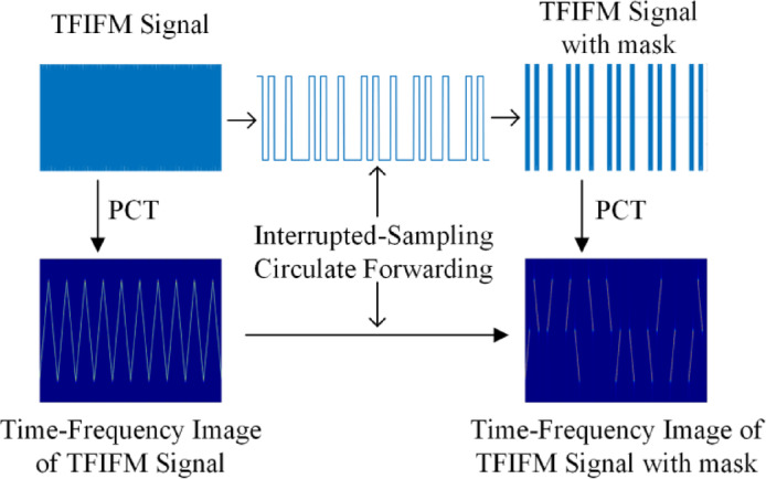
The masking effect of the interrupted sampling on time–frequency images of proximity detector signals.
Classification model
Constructing the AMC model based on TFRNet and adaptive random mask algorithm
The process and model structure of the AMC method are shown in Fig. 3. The TFRNet model uses a structure consisting of an encoder, decoder, and classification module. The encoder and decoder consist of different layers of a Transformer based on the multi-head attention mechanism. The classification module primarily comprises a global average pooling layer, a Dense layer, and a Softmax activation function. The signal processing process of the AMC method based on TFRNet and the adaptive random mask algorithm is as follows.
Fig. 3.

Process and network structure of the proposed AMC method.
The proximity detector signals  are first obtained via IS
  , and the signals are subsequently transformed into TFI
  via the TF analysis
  .
.
 |
6 |
The input images are partitioned into equal-sized image patches, and each patch is positionally encoded. Then, mask elimination is performed on some patches. The mask matrix is defined as  . Here,
  is a n*n matrix.
 |
7 |
An adaptive random mask algorithm is proposed for the TFI of proximity detector signals to improve the computational efficiency and reconstruction effect. The adaptive random mask algorithm flow is shown in Fig. 4 and Algorithm 1.
Fig. 4.
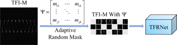
Schematic diagram of the adaptive random mask algorithm.
Algorithm 1.

Adaptive random mask algorithm
The adaptive random mask algorithm obtains the threshold comparison result of each image patch relative to the whole TFI by segmenting and thresholding the TFI of the proximity detector signal. The invalid image patches are removed adaptively according to the threshold comparison result, to concentrate the attention area of the model into the effective area containing TF features and improve the computational efficiency. With the help of a random mask, the feature information is randomly eliminated to prevent the model from falling into overfitting, to improve the generalization performance of the model, and to extend its learning ability. Adaptive random mask algorithm also makes the model focus only on the characteristics of the input itself by masking, without the need to train with the help of labels and other information, thus realizing self-supervised learning and providing support for pre-training of the model and fine-tuning of small sample sizes. After masking the TFI of the IS proximity detector signals by the adaptive random mask algorithm, the AMC is further carried out in the TFRNet model. The processing of the TFRNet model is shown in Algorithm 2.
Algorithm 2.

TFRNet classification algorithm
As shown in Algorithm 2, after the TFI has been masked, the remaining image patches are mapped onto one-dimensional vectors by a convolutional layer to form multiple sets of one-dimensional tokens, and a class token (CLS) with the same size as the individual token is set up. The CLS is used as input to the classification module. The position encoding information is included in the tokens. The tokens, the position encoding information, and the CLS are fed together into the encoder. The encoder extracts features from the tokens and outputs a feature map with a constant size. The feature map output by the encoder is zero-complemented by position coding and then input into the decoder, which reconstructs the TFI based on the feature map and position coding information and outputs the CLS. The CLS is processed by the classification module using global average pooling, fully connected unfolding, and smoothing to generate the final modulation type vector for the IS proximity detector signal.
Self-supervised pretraining and transfer learning for the AMC model
The training method of the TFRNet model is shown in Algorithm 3, which can be divided into the following steps. First, the self-supervised pretraining process of the TFRNet model is realized using unlabeled proximity detector signals with a complete TF domain. Only the encoder and decoder are trained for TF reconstruction. The pretraining samples are obtained via simulation. Then, by transfer learning, the whole TFRNet model is trained for fine-tuning classification using a small number of IS proximity detector signals. The samples used for the fine-tuning classification process are truncated proximity detector signals in the TF domain obtained by sampling in an actual proximity detector jamming instrument.
Algorithm 3.

Self-supervised pretraining and transfer learning algorithm
Loss functions and optimization algorithms
During pretraining, the mean square error (MSE) loss is utilized. This metric evaluates the extent of deviation between the predicted and actual values, as illustrated in Eq. (8), which is adapted from the standard formulation49.
 |
8 |
where  denotes the actual value and
  denotes the predicted value.
The cross-entropy loss, employed for refining classification accuracy, quantifies the discrepancy between actual and predicted labels. The mathematical expression for this loss function is provided in Eq. (9), which is adapted from the standard formulation50.
 |
9 |
where  denotes the actual label and
  denotes the predicted label.
Computational efficiency analysis
The computational complexity of PCT is mainly composed of sliding window processing and FFT calculations. Suppose the signal length is  , the window length is
  , and the number of frequency points is
  . In the sliding window processing, the operation is repeated
  times, with each iteration having a complexity of
  . Therefore, the overall computational complexity is
  . In the FFT computation, the FFT is performed on
  columns, each with
  points, resulting in a computational complexity of
  . Therefore, the overall computational complexity of PCT is
  .
.
The encoder and decoder of the asymmetric structure of TFRNet consist of a Transformer architecture. The time computational complexity of the Transformer mainly depends on the multi-head attention and feed-forward neural network.
For multi-head attention, assume that there are  heads. Simplify the dimensions of the query, key, and value matrices are
  .
.  is the number of sequence elements.
  is the representation dimension. Ignore the effect of constant coefficients.
Then computing the query, key, and value matrix as  with
with  gives a computational complexity of
  . Calculating both similarity and weighted sum as
  with
with  operation, the computational complexity is
  . The complexity of the output linear mapping is
  for the operation of
  and
and  . Therefore, the computational complexity of the multi-head attention is
  .
.
Assuming that the hidden layer dimension is  . A feedforward neural network usually consists of two linear transformations and an activation function, and the operation is
  +
+  the computational complexity is
  .
.
Therefore, the computational complexity of Transformer based on multi-head attention is  . Consider that the encoder has
  layers and the decoder has
  layers. Then the encoder and decoder computational complexity is
  .
.
The computational complexity of the classification module mainly depends on the Dense layer and the Softmax activation function. The Dense layer performs multiplication and summation operations with  computational complexity, while the Softmax activation function performs exponentiation, summation, and division operations with
  . The L2 paradigm is computed by calculating the square of each element, summing and taking the square root of the sum, with a total complexity of
  . Therefore, the computational complexity of the TFRNet model is
  .
.
Experimental results
Experimental scenario and parameter settings
Five different modulation types of proximity detector signals were selected for classification in this study. The modulation of the proximity detector signals includes the TRIFM, the sine-wave FM (SINFM), the linear FM pulse compression (LFMPC), the pseudocode phase modulation (PSD), and the pseudocode phase-modulated pulse doppler composite (PSPD). The proximity detector signals are acquired by IS, and the TF analysis is then used to acquire the TFI of the proximity detector signals. The signal data used in the experiments were acquired in a microwave darkroom through the data acquisition and analysis system. The experimental scenario of the microwave darkroom is shown in Fig. 5.
Fig. 5.
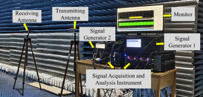
Experimental scenario.
The data acquisition and analysis system primarily consists of the signal generator, antenna, and signal acquisition and analysis instrument. The experimental principle is shown in Fig. 6.
Fig. 6.
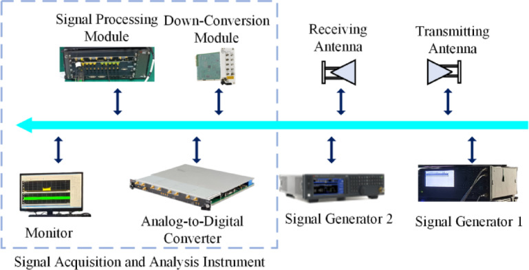
Experimental Principle.
The signal generator 1 is connected to the transmitting antenna to transmit proximity detector signals of different modulation types. The signal acquisition and analysis instrument is connected to the receiving antenna and receives the proximity detector signals according to different IS strategies in the actual working process. The signal generator 2 is the fundamental oscillator of the signal acquisition and analysis instrument. The signal acquisition and analysis instrument mainly includes a down-conversion module, an analog-to-digital converter (ADC), a high-speed signal processing module, an embedded PC, and a monitor. After the receiving antenna receives the radio frequency (RF) proximity detector signal by the IS strategy, the RF signal is mixed into an intermediate frequency (IF) signal by the fundamental oscillator and the down-conversion module, then converted into an IF digital signal by the ADC and transferred into a high-speed signal processing module and an embedded PC to carry out classification and recognition processing. The monitor displays the time domain and frequency spectrum of the received proximity detector signal in real time. The sampling rate of the proximity detector signal in the experiment is 400 MHz. Some parameters of the instrument are shown in Table 1.
Table 1.
The major hardware and parameters of the data acquisition and analysis system.
| Module | Parameter |
|---|---|
| Down-Conversion Module |
10 MHz ~ 50 GHz Bandwidth 1.5 GHz |
| Signal Generator 1 | 250 kHz ~ 44 GHz |
| Signal Generator 2 | 9 kHz ~ 40 GHz |
| Analog-to-Digital Converter | 12-bit and Fs > = 1 GHz |
| Transmitting Antenna | 10–40 GHz |
| Receiving Antenna | 10–40 GHz |
The detailed parameter configurations for various proximity detector signals are presented in Table 2, where MF denotes the modulation frequency, FD denotes the frequency deviation, PW denotes the pulse width, EW denotes the codeword width, and DC denotes the duty cycle.
Table 2.
Parameters of different proximity detector signals.
| Modulation Type |
MF (KHz) | FD (MHz) |
PW (ns) |
EW (ns) |
DC |
|---|---|---|---|---|---|
| TRIFM | [50, 100] | [50, 150] | – | – | – |
| SINFM | [50, 100] | [50, 150] | – | – | – |
| LFMPC | [50, 100] | [50, 150] | [1e3, 1e4] | – | [40, 50] |
| PSD | – | – | – | [50, 500] | – |
| PSPD | – | – | [10, 250] | [50, 500] | [20, 50] |
Table 3 displays the parameter configurations for the IS process, with the following notations: ST represents the duration of a single sampling operation, FT signifies the time needed for a single forwarding operation, SD stands for the sampling duration, NS indicates the number of samples, and NF reflects the number of forwarding operations. Boxes in the table indicate range values, including maximum and minimum values.
Table 3.
Parameters of different interrupted sampling modes.
| Mode | ST (us) | FT (us) | SD (us) | NS | NF | DC |
|---|---|---|---|---|---|---|
| Direct | [1, 5] | [1, 5] | 200 | 1 | 1 | 50 |
| Repeat | [1, 5] | [1, 5] | 200 | 1 | 3 | 25 |
| Circulate | [1, 5] | [1, 5] | 200 | 1 | 1, 2, 3 | 33.3 |
Table 4 summarizes the key hyperparameters of the PCT-TFRNet model, including learning rate, batch size, optimizer settings, and network architecture details. These values were selected to optimize performance and ensure reproducibility.
Table 4.
Hyperparameters of the PCT-TFRNet Model.
| Hyperparameter | Value | Description |
|---|---|---|
| FLevel | 1024 | The number of frequency points in PCT |
| WinLen | 512 | The Gaussian window length of PCT |
| Alpha | 5 | The chirp rate of PCT. (Hz/s) |
| Patch Size | 14 | The size of the patch into which the TFI is divided |
| Encoder Layers | 12 | The number of layers in the Transformer encoder |
| Encoder Multi-Head Attention Heads | 12 | The number of heads in the multi-head attention of the encoder |
| Encoder Hidden Dimension | 588 | The hidden layer dimension of the encoder |
| Decoder Layers | 8 | The number of layers in the Transformer decoder |
| Decoder Multi-Head Attention Heads | 16 | The number of heads in the multi-head attention of the decoder |
| Decoder Hidden Dimension | 512 | The hidden layer dimension of the decoder |
| Learning Rate | 0.001 | Initial learning rate |
| Batch Size | 32 | The batch size used for training |
| Epoch | 50 | Fine-tuning epochs |
| Train/Test Ratio | 4:1 | Training-to-testing dataset ratio |
| Optimizer |
AdamW ( |
Optimizer used for training |

Time-frequency reconstruction
During the time–frequency reconstruction pretraining process, the encoder and decoder of the TFRNet model are trained using unlabeled TFI-O data with complete time–frequency distributions generated through simulations. Three modulation types for SINFM, TRIFM, and LFMPC proximity detector signals are selected for the TF reconstruction demonstration. The TF reconstruction effect of the TFRNet model is shown in Fig. 7. The type of IS proximity detector signal sample used for the pretraining process is TFI-O, and the fine-tuning classification process uses TFI-M.
Fig. 7.
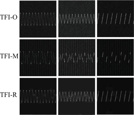
Effect of time–frequency reconstruction with an SNR of −5 dB.
Figure 7 shows that the TFRNet model can reconstruct the TF distributions of signals possessing different modulation types at low SNRs. The difference between the TF distribution characteristics of TFI-O and TFI-R is very small, which shows that the TFRNet model can completely reconstruct the signal characteristics, including the period, bandwidth, and slope. The reconstruction process also remains effective when the SNR is low.
Fine-tuning classification training and robustness analysis
The TFRNet model was fine-tuned for classification tasks using an experimental training dataset, which was divided into three sub-datasets according to signal forwarding modes: Direct forwarding, Repeat forwarding, and Circulate forwarding. Each modulation type of the IS proximity detector signals contains 200 training samples, 50 testing samples, and 100 validation samples within each sub-dataset. The SNR conditions range from −15 to 0 dB, with a step size of 1 dB, reflecting the low-SNR environments typically encountered in real-world IS applications. The training process was conducted over 50 epochs, which was determined based on convergence behavior and to balance learning adequacy with overfitting prevention in small-sample scenarios.
Table 5 presents the classification performance of the PCT-TFRNet framework across distinct IS modes, detailing accuracy metrics for various signal modulation types in the validation dataset. The reported values represent SNR-averaged measurements calculated across the −15 to 0 dB SNR range.
Table 5.
The classification accuracy (%) achieved by PCT-TFRNet on the validation dataset.
| Mode | LFMPC | PSD | PSPD | SINFM | TRIFM | AVERAGE |
|---|---|---|---|---|---|---|
| Direct | 99.47 | 99.73 | 99.51 | 98.34 | 99.82 | 99.37 |
| Repeat | 95.89 | 98.96 | 97.87 | 96.97 | 98.55 | 97.65 |
| Circulate | 99.57 | 99.68 | 99.73 | 95.72 | 99.94 | 98.93 |
As shown in Table 5, the TFRNet model demonstrates strong robustness and high classification performance, performing best in direct forwarding mode, followed by circulate forwarding. This confirms the effectiveness of the proposed TFRNet-based AMC method with transfer learning for small-sample IS scenarios, enabling accurate modulation recognition of IS proximity detector signals.
Ablation study: comparison of different TF analysis methods and comparison of asymmetric and symmetric encoder-decoder structures
Ablation study systematically evaluates the contribution of each component to a model’s performance by removing or modifying parts of the model. In this study, we designed two separate ablation experiments: one for comparing different TF analysis methods and the other for comparing asymmetric and symmetric encoder-decoder structures.
First, TF analysis, as a signal preprocessing method for AMC, directly impacts classification performance due to its accuracy in extracting TF features. Therefore, the first experiment compares the classification performance of STFT, SPWVD, and PCT under different IS modes, aiming to evaluate the effect of different TF analysis methods on classification accuracy. The second experiment focuses on comparing the impact of asymmetric and symmetric encoder-decoder structures on model performance to validate the advantages of the asymmetric encoder-decoder structure.
To evaluate the performance of the TFRNet model, the performance evaluation dataset was collected by introducing noise and augmented data during the experiments, and still included three sub-datasets for different IS modes. The SNR range for each sub-dataset is from −16 to 4 dB, increasing in 2 dB steps, with 500 data samples of a single modulation type available at each SNR level.
Figure 8 demonstrates that the classification performance of the TFRNet model varies significantly when different TF analyses are employed as signal preprocessing steps in various IS modes. For SNR values above −8 dB, the classification performance of various TF analysis methods shows minimal variation. Consequently, the figure only highlights the sections where significant differences are observed.
Fig. 8.

Comparison curves of classification accuracy of TF analysis methods for TFRNet under different interrupted sampling modes. (a) Direct. (b) Repeat. (c) Circulate.
The performance gap between the SPWVD-TFRNet, the PCT-TFRNet, and the STFT-TFRNet is significant, indicating that the classification curve and performance metrics of the STFT-TFRNet model are significantly lower than those of the former two. This is because the STFT has a fixed window length and is insensitive to changes in signal characteristics. Moreover, the resolutions in the time and frequency dimensions are limited to each other, and the TF resolution is unevenly distributed. This leads to poor TF feature differentiation of the signal extracted by the STFT, which reduces the classification accuracy.
The accuracy curves between the PCT-TFRNet and SPWVD-TFRNet are closer, and the gap in classification performance is smaller. As shown in Fig. 8a, the classification performance of the two methods is almost the same in the direct modes. The SPWVD utilizes the dual-window mechanism to independently adjust the smoothing parameter and resolution of the time domain and the frequency dimension, which enhances the TF distribution aggregation of the signal and improves the differentiation of the TF features, achieving good classification results.
The PCT enhances the TF resolution and feature localization ability by replacing the traditional linear FM kernel with a polynomial waveform structure, which can better characterize the signal features. The polynomial waveform structure can better describe the continuous transformation of the signal by utilizing the Weierstrass approximation theorem51, which leads to higher energy aggregation and thus better classification performance. Therefore, according to the results of the ablation experiments shown in Fig. 8, the use of PCT as a signal preprocessing method in the AMC method based on the TFRNet model has the best classification performance.
Figure 9 illustrates the classification accuracy of two encoder-decoder structures. The asymmetric model corresponds to PCT-TFRNet, while the symmetric model adopts the same encoder-decoder configuration, both with 12-layer transformers and 12 attention heads. When the SNR is above -8 dB, the performance difference between the two models is negligible. Therefore, the histogram highlights only the SNR range where noticeable differences occur. As shown, the asymmetric structure consistently outperforms the symmetric one, particularly under low-SNR conditions, demonstrating superior robustness. This performance trend remains consistent across all three IS modes.
Fig. 9.

Classification accuracy comparison of asymmetric and symmetric structures under different interrupted sampling modes. (a) Direct. (b) Repeat. (c) Circulate.
The results show that the asymmetric encoder-decoder structure enhances classification accuracy, particularly in low-SNR conditions. It improves model robustness and performance, making it a valuable component of the TFRNet architecture.
Classification performance comparison
To comprehensively evaluate the classification performance of the proposed method, systematic analysis, and comparative evaluations were conducted from multiple dimensions, including classification accuracy across different modulation-type signals, as well as performance comparisons with state-of-the-art models under low SNR conditions and small-sample scenarios. Unless otherwise specified, the models are trained using the experimental training dataset and evaluated using the performance evaluation dataset. The training period is 50.
Classification for different modulation types of signals
Figure 10 shows the classification accuracy curves of the PCT-TFRNet model for different signal modulation types across various SNR levels. Figure 10 indicates that, within the SNR range from −16 to −12 dB, the classification accuracy of the PCT-TFRNet model for different modulation types increases noticeably as SNR improves. Above −10 dB SNR, the PCT-TFRNet achieves classification accuracies over 95%. The figure focuses solely on the sections where significant differences in performance are evident.
Fig. 10.

Classification accuracy curves of the PCT-TFRNet model for various modulation types of signals at different SNRs. (a) Direct. (b) Repeat. (c) Circulate.
As illustrated in Fig. 10, the classification performance of PCT-TFRNet for different modulation-type signals exhibits significant variations under distinct IS modes. In low SNR conditions, the classification accuracy for LFMPC and SINFM proximity detector signals is notably inferior compared to other signal types. This indicates that IS causes more severe distortion to the TF characteristics of these two specific signals. Particularly under the repeat forwarding mode, the classification effectiveness for all signal categories remains lower than in the other two operational modes. This suggests that this forwarding pattern induces a more substantial degradation of signal TF features. However, with progressive improvement in SNR levels, the model demonstrates robust classification capabilities exceeding 95% accuracy across all signal types. Therefore, the proposed method has excellent classification performance for different types of signals when the SNR is more desirable.
Comparison with other methods at low SNR
To rigorously evaluate the classification efficacy of the TFRNet models, 50 epochs were trained on all models using the same parameters. The AMC models used for this comparison include DLRNet37, DenseNet-F2230, MLResNet39, VGG-1131, and MLCNN40. The classification accuracy curves produced by the different models under various SNRs are presented in Fig. 11, Tables 6, and 7.
Fig. 11.

Curves of the classification accuracy versus the SNR for different interrupted sampling modes. (a) Direct. (b) Repeat. (c) Circulate.
Table 6.
The classification accuracy (%) of different AMC models with partial SNRs.
| IS Mode | Direct | Repeat | Circulate | ||||||
|---|---|---|---|---|---|---|---|---|---|
| SNR (dB) | −16 | −14 | −12 | −16 | −14 | −12 | −16 | −14 | −12 |
| PCT-TFRNet (ours) | 83.1 | 96.8 | 99.2 | 70.2 | 89.9 | 97.4 | 74.0 | 92.5 | 98.9 |
| DLRNet37 | 66.6 | 83.1 | 95.6 | 57.2 | 79.6 | 92.9 | 57.6 | 77.9 | 89.9 |
| DenseNet-F2230 | 64.4 | 83.3 | 94.5 | 48.6 | 76.8 | 90.5 | 50.4 | 74.6 | 88.8 |
| MLResNet39 | 62.8 | 81.7 | 93.2 | 59.3 | 77.6 | 89.7 | 55.9 | 77.8 | 89.9 |
| VGG-1131 | 69.5 | 82.0 | 95.9 | 57.0 | 80.0 | 92.7 | 58.1 | 72.3 | 85.4 |
| MLCNN40 | 44.8 | 69.8 | 87.7 | 39.0 | 64.7 | 82.3 | 43.2 | 69.1 | 84.6 |
Table 7.
Classification results of different AMC models under IS modes.
| IS Mode | Model | Accuracy (%) | Precision (%) | Recall (%) | F1-Score |
|---|---|---|---|---|---|
| Direct | PCT-TFRNet (ours) | 98.06 | 98.45 | 97.99 | 0.982 |
| DLRNet37 | 94.37 | 95.02 | 94.09 | 0.946 | |
| DenseNet-F2230 | 94.06 | 94.77 | 94.14 | 0.945 | |
| MLResNet39 | 93.79 | 94.31 | 93.69 | 0.940 | |
| VGG-1131 | 94.92 | 95.42 | 94.93 | 0.952 | |
| MLCNN40 | 89.48 | 90.31 | 89.78 | 0.900 | |
| Repeat | PCT-TFRNet (ours) | 95.59 | 97.13 | 95.64 | 0.964 |
| DLRNet37 | 92.28 | 93.75 | 92.81 | 0.933 | |
| DenseNet-F2230 | 90.82 | 92.31 | 91.69 | 0.920 | |
| MLResNet39 | 91.58 | 93.06 | 92.40 | 0.927 | |
| VGG-1131 | 92.35 | 93.92 | 92.81 | 0.936 | |
| MLCNN40 | 85.73 | 87.39 | 85.82 | 0.866 | |
| Circulate | PCT-TFRNet (ours) | 96.82 | 97.29 | 96.78 | 0.970 |
| DLRNet37 | 92.20 | 93.10 | 92.42 | 0.928 | |
| DenseNet-F2230 | 91.55 | 92.24 | 91.57 | 0.919 | |
| MLResNet39 | 92.25 | 93.14 | 92.54 | 0.928 | |
| VGG-1131 | 90.60 | 91.47 | 90.91 | 0.912 | |
| MLCNN40 | 87.62 | 88.77 | 88.16 | 0.885 |
As illustrated in Fig. 11 and Table 6, the proposed PCT-TFRNet model demonstrates superior classification accuracy compared to the other AMC models, particularly within the SNR range from −16 to −12 dB. When operating at an SNR of −16 dB, the PCT-TFRNet model demonstrates classification accuracy rates that surpass state-of-the-art counterparts by more than 10 percentage points across all IS modes. The experimental results conclusively demonstrate the robustness and advancement of the proposed method under varying SNR conditions. Notably, the performance superiority of the proposed method becomes more pronounced as the SNR decreases.
To provide a more comprehensive and objective assessment of the PCT-TFRNet model’s classification performance, we complement overall accuracy with additional standard evaluation metrics, including precision, recall, and F1-score. These metrics are particularly valuable for evaluating performance under imbalanced or noisy signal conditions, as they reveal the trade-offs between false positives and false negatives. Table 7 reports these metrics, accuracy, precision, recall, and F1-score, averaged over the full SNR range from −16 to 4 dB in 2 dB increments. The results are presented for the three IS modes: Direct, Repeat, and Circulate.
As observed, the proposed PCT-TFRNet achieves consistently high precision and recall across all IS modes, demonstrating strong robustness under low-SNR and fragmented signal conditions. Its F1-score remains above 0.96 in all scenarios, clearly outperforming other models. This indicates that PCT-TFRNet strikes a better balance between precision and recall, leading to more reliable classification compared to existing methods.
Comparison with other methods in small samples
In this section, to validate the performance of the proposed method in small-sample learning scenarios, a reduction in the number of training samples is used to train the classification model and evaluate its classification performance. The number of training samples for each modulation type proximity detector signal was progressively scaled down from 200 to 50 and evaluated using the performance validation dataset, and the results obtained are shown in Figs. 12 and 13. Among them, Fig. 12 demonstrates the trends of the classification performance of the PCT-TFRNet model in different IS modes with the reduction of the number of training samples under SNR of −10, −12, −14, and −16 dB, respectively. Figure 13 demonstrates the trends of the classification performance of the proposed method in different IS modes with a decreasing number of training samples in comparison with the state-of-the-art model when the SNR is −14 dB.
Fig. 12.

The trend of classification performance of PCT-TFRNet with decreasing number of training samples at different SNR. (a) − 10 dB (b) − 12 dB (c) − 14 dB (d) − 16 dB.
Fig. 13.

The trend of classification accuracy of the compared methods with the number of training samples at an SNR of − 14 dB. (a) Direct. (b) Repeat. (c) Circulate.
As shown in Fig. 12, when the number of training samples for each modulation type is reduced from 200 to 50, the maximum classification accuracy degradation values are approximately 0.026 at −10 dB, 0.042 at −12 dB, 0.09 at −14 dB, and 0.12 at −16 dB. The PCT-TFRNet model shows the most significant performance degradation in repeat forwarding mode. This observation confirms previous experimental conclusions that repeat forwarding mode captures the most defective signal characteristics and is most likely to cause signal distortion.
However, as seen in Fig. 12, although the classification performance of PCT-TFRNet demonstrates a decreasing trend with reduced training samples, the decline rate remains gradual. Specifically, higher SNR levels correspond to smaller impacts from training sample reduction. This indicates that under ideal SNR conditions, PCT-TFRNet can achieve training convergence rapidly with very few samples, effectively reducing dependence on actual training data while maintaining desirable performance in small-sample learning scenarios.
As evidenced in Fig. 13, state-of-the-art methods exhibit progressively amplified classification performance degradation as training samples diminish, with degradation severity positively correlating with increasing SNR levels. This phenomenon confirms these methods’ inherent constraints in attaining model convergence under limited training data conditions, particularly exacerbated in low-SNR regimes where maximum accuracy deterioration occurs. On the other hand, the proposed method can significantly improve the extraction of signal features by TFRNet and reduce the dependence on actual training samples. The experimental results conclusively show that PCT-TFRNet outperforms in classification across all IS modes, with notably less performance decline during sample reduction, quantitatively confirming its increased robustness compared to traditional methods.
Based on the above experimental and performance analysis results, the proposed PCT-TFRNet model performs significantly better in classification than similar methods in low SNR and small sample learning scenarios. The reasons behind these results can be divided into three aspects.
The signal preprocessing method based on PCT has superior signal feature representation ability compared to other TF analysis methods or two-dimensional signal transformations. PCT can not only accurately describe the instantaneous change of signals but also achieve some noise reduction, significantly improving feature extraction and classification in the subsequent TFRNet model.
During the IS process, signals lose some modulation features, and these features diminish further as SNR declines, which hampers classification. However, the PCT-TFRNet model can adaptively learn the underlying laws of IS proximity detector signals and reconstruct their TF features through random masking and self-supervised pretraining. This allows IS signals to be recognized even at low SNRs.
The limited number of actual IS proximity detector signals restricts the classification capabilities of the compared methods. We propose using a self-supervised pretraining approach combined with a transfer learning framework to expand the internal representations learned from IS signals by leveraging the pretrained TFRNet model. As a result, the PCT-TFRNet model can achieve improved classification performance even with a restricted sample size.
Conclusion
This paper proposes a novel method based on PCT and TFRNet for modulation classification of IS proximity detector signals with limited sample sizes. The method is designed for proximity detector jamming instruments under adversarial conditions. PCT is a signal preprocessing technique to enhance the separability of TF features. The TFRNet model, constructed with an asymmetric encoder-decoder architecture, integrates an adaptive random mask algorithm to reconstruct complete TF representations from signals affected by IS, even under low SNR conditions. The model incorporates self-supervised learning and transfer learning strategies to address the challenge of limited samples. Extensive experiments evaluated the proposed approach’s performance under varying SNR levels, different IS modes, and small-sample learning scenarios. Additional ablation studies were performed to assess the effectiveness of different TF analysis methods and compare the performance of asymmetric and symmetric encoder-decoder structures. Experimental results demonstrate that the PCT-based preprocessing significantly improves the representation of TF features. Compared to other state-of-the-art methods, the PCT-TFRNet framework, enhanced with transfer learning and adaptive masking, achieves superior classification performance and robustness in low SNR and small-sample scenarios. Notably, it achieves over 89% classification accuracy at SNR levels above -14 dB, confirming its effectiveness and practical applicability for modulation type recognition of IS proximity detector signals.
Acknowledgements
National Natural Science Foundation of China under Grant No. 62301051.
Author contributions
Guanghua Yi was responsible for theoretical analysis, methodology design, and simulation verification, while Xinhong Hao and Xiaopeng Yan provided conceptual guidance and methodological advice for the study. Jian Dai oversaw the overall coordination of the research and experiments. Guanghua Yi and Yongzhou Wang were responsible for experimental data collection and validation. Guanghua Yi drafted the manuscript with contributions from Yongzhou Wang and Dan Hu. The revision of the manuscript was primarily carried out by Guanghua Yi, Jian Dai, and Xiaopeng Yan, with assistance from the other authors. All authors have read and agreed to the published version of the manuscript.
Declarations
Competing interests
The authors declare no competing interests.
Data availability
The datasets generated during or analyzed during the current study are available from the corresponding author on reasonable request.
Footnotes
Publisher’s note
Springer Nature remains neutral with regard to jurisdictional claims in published maps and institutional affiliations.
Xinhong Hao and Xiaopeng Yan have contributed equally to this work.
Contributor Information
Xiaopeng Yan, Email: yanxiaopeng@bit.edu.cn.
Jian Dai, Email: jiandai@bit.edu.cn.
References
- 1.Zhang, L., Lambotharan, S., Zheng, G., AsSadhan, B. & Roli, F. Countermeasures against adversarial examples in radio signal classification. IEEE Wirel Commun Lett10, 1830–1834 (2021). [Google Scholar]
- 2.Qi, P., Zhou, X., Zheng, S. & Li, Z. Automatic modulation classification based on deep residual networks with multimodal information. IEEE Trans Cognitive Commun Netw7, 21–33 (2021). [Google Scholar]
- 3.Kumar, A. & Manish, S. U. Residual stack-aided hybrid CNN-LSTM-based automatic modulation classification for orthogonal time-frequency space system. IEEE Commun Lett27, 3255–3259 (2023). [Google Scholar]
- 4.Fu, X., Gui, G., Wang, Y., Gacanin, H. & Adachi, F. Automatic modulation classification based on decentralized learning and ensemble learning. IEEE Trans. Veh. Technol.71, 7942–7946 (2022). [Google Scholar]
- 5.Zhang, X. et al. Lightweight automatic modulation classification via progressive differentiable architecture search. IEEE Trans Cognitive Commun Netw9, 1519–1530 (2023). [Google Scholar]
- 6.Huang, S., Jiang, Y., Gao, Y., Feng, Z. & Zhang, P. Automatic modulation classification using contrastive fully convolutional network. IEEE Wirel Commun Lett8, 1044–1047 (2019). [Google Scholar]
- 7.Zhang, H., Zhou, F., Wu, Q., Wu, W. & Hu, R. Q. A novel automatic modulation classification scheme based on multi-scale networks. IEEE Trans Cognitive Commun Netw8, 97–110 (2022). [Google Scholar]
- 8.Zheng, J. & Wei, G. New Development of electromagnetic compatibility in the future: Cognitive Electromagnetic environment adaptation. In 2021 13th Global Symposium on Millimeter-Waves & Terahertz (GSMM), 1–3 (2021).
- 9.Dai, J., Hao, X., Liu, Q., Yan, X. & Li, P. Repeater jamming suppression method for pulse Doppler fuze based on identity recognition and chaotic encryption. Defence Technology17, 1002–1012 (2021). [Google Scholar]
- 10.Luan, S., Gao, Y., Zhou, J. & Zhang, Z. Automatic modulation classification based on Cauchy-score constellation and lightweight network under impulsive noise. IEEE Wirel Commun Lett10, 2509–2513 (2021). [Google Scholar]
- 11.Hanbali, B. S. S. Technique to counter improved active echo cancellation based on ISRJ with frequency shifting. IEEE Sens J19, 9194–9199 (2019). [Google Scholar]
- 12.Yi, G., Hao, X., Yan, X., Wang, J. & Dai, J. Automatic modulation recognition for radio frequency proximity sensor signals based on masked autoencoders and transfer learning. IEEE Trans. Aerosp. Electron. Syst.60, 8700–8712 (2024). [Google Scholar]
- 13.Zhang, P., Huang, Y. & Jin, Z. A New Electronic jamming method inspried from bionics system. In 2020 IEEE 5th international conference on signal and image processing (ICSIP) 572–576 (2020).
- 14.Wu, Q., Liu, J., Wang, J., Zhao, F. & Xiao, S. Improved active echo cancellation against synthetic aperture radar based on nonperiodic interrupted sampling modulation. IEEE Sens. J.18, 4453–4461 (2018). [Google Scholar]
- 15.Li, J., Dai, J., Hao, X., Yan, X. & Wang, X. Air target recognition method against ISRJ for radio frequency proximity sensors using chaotic stream encryption. Def Technol28, 267–279 (2023). [Google Scholar]
- 16.Dai, J., Hao, X., Yan, X. & Li, Z. Adaptive false-target recognition for the proximity sensor based on joint-feature extraction and chaotic encryption. IEEE Sens. J.22, 10828–10840 (2022). [Google Scholar]
- 17.Bahloul, M. R., Yusoff, M. Z., Abdel-Aty, A.-H. & Saad, M. N. M. An efficient likelihood-based modulation classification algorithm for MIMO systems. J. Comput. Theor. Nanosci.13, 7879–7885 (2016). [Google Scholar]
- 18.Abdul Salam, A. O., Sheriff, R. E., Al-Araji, S. R., Mezher, K. & Nasir, Q. A unified practical approach to modulation classification in cognitive radio using likelihood-based techniques. In 2015 IEEE 28th Canadian Conference on Electrical and Computer Engineering (CCECE) 1024–1029 (2015).
- 19.Xu, J. L., Su, W. & Zhou, M. Likelihood-ratio approaches to automatic modulation classification. IEEE Trans Syst, Man, Cybern, Part C41, 455–469 (2011). [Google Scholar]
- 20.Zhu, D., Mathews, V. J. & Detienne, D. H. A Likelihood-based algorithm for blind identification of QAM and PSK signals. IEEE Trans. Wireless Commun.17, 3417–3430 (2018). [Google Scholar]
- 21.Ramezani-Kebrya, A., Kim, I.-M., Kim, D. I., Chan, F. & Inkol, R. Likelihood-based modulation classification for multiple-antenna receiver. IEEE Trans. Commun.61, 3816–3829 (2013). [Google Scholar]
- 22.Güner, A., Alçin, Ö. F. & Şengür, A. Automatic digital modulation classification using extreme learning machine with local binary pattern histogram features. Measurement145, 214–225 (2019). [Google Scholar]
- 23.Wang, Y. et al. Federated learning for automatic modulation classification under class imbalance and varying noise condition. IEEE Trans Cognitive Commun Netw8, 86–96 (2022). [Google Scholar]
- 24.Guo, Q., Nan, P. & Wan, J. Signal classification method based on data mining for multi-mode radar. J. Syst. Eng. Electron.27, 1010–1017 (2016). [Google Scholar]
- 25.Xiang, Y. & Hong-yu, Gu. A signal sorting algorithm based on time difference of arrival. Histogram. J Electron Inf Technol37, 2762–2768 (2015). [Google Scholar]
- 26.Hussain, A. et al. Automatic modulation recognition based on the optimized linear combination of higher-order cumulants. Sensors22(19), 7488 (2022). [DOI] [PMC free article] [PubMed] [Google Scholar]
- 27.Liu, S., Yan, X., Li, P., Hao, X. & Wang, K. Radar emitter recognition based on SIFT position and scale features. IEEE Trans. Circuits Syst. II Express Briefs65, 2062–2066 (2018). [Google Scholar]
- 28.Chu, P., Xie, L., Dai, C. & Chen, Y. Automatic modulation recognition for secondary modulated signals. IEEE Wirel Commun Lett10, 962–965 (2021). [Google Scholar]
- 29.Che, J., Wang, L., Bai, X., Liu, C. & Zhou, F. Spatial-temporal hybrid feature extraction network for few-shot automatic modulation classification. IEEE Trans. Veh. Technol.71, 13387–13392 (2022). [Google Scholar]
- 30.Liu, Y., Yan, X., Hao, X., Yi, G. & Huang, D. Automatic modulation recognition of radiation source signals based on data rearrangement and the 2D FFT. Remote Sens15(2), 518 (2023). [Google Scholar]
- 31.Simonyan, K. & Zisserman, A. Very deep convolutional networks for large-scale image recognition. In: 3rd International conference on learning representations, ICLR 2015, San Diego, CA, USA, May 7–9, 2015, conference track proceedings (eds. Bengio, Y. & LeCun, Y.) (2015).
- 32.Hermawan, A. P., Ginanjar, R. R., Kim, D.-S. & Lee, J.-M. CNN-based automatic modulation classification for beyond 5G communications. IEEE Commun. Lett.24, 1038–1041 (2020). [Google Scholar]
- 33.Hong, D., Zhang, Z. & Xu, X. Automatic modulation classification using recurrent neural networks. In: 2017 3rd IEEE International conference on computer and communications (ICCC) 695–700 (2017).
- 34.Rajendran, S., Meert, W., Giustiniano, D., Lenders, V. & Pollin, S. Deep learning models for wireless signal classification with distributed low-cost spectrum sensors. IEEE Trans Cognitive Commun Netw4, 433–445 (2018). [Google Scholar]
- 35.Ma, J. et al. Automatic modulation classification in impulsive noise: Hyperbolic-tangent cyclic spectrum and multibranch attention shuffle network. IEEE Trans. Instrum. Meas.72, 1–13 (2023).37323850 [Google Scholar]
- 36.Chen, K., Zhu, L., Chen, S., Zhang, S. & Zhao, H. Deep residual learning in modulation recognition of radar signals using higher-order spectral distribution. Measurement185, 109945 (2021). [Google Scholar]
- 37.Yi, G. et al. Automatic modulation recognition of radiation source signals based on two-dimensional data matrix and improved residual neural network. Def Technol33, 364–373 (2024). [Google Scholar]
- 38.Walenczykowska, M., Kawalec, A. & Krenc, K. An application of analytic wavelet transform and convolutional neural network for radar intrapulse modulation recognition. Sensors23(4), 1986 (2023). [DOI] [PMC free article] [PubMed] [Google Scholar]
- 39.Hong-hai, Y., Xiao-peng, Y., Shao-kun, L., Ping, L. & Xin-hong, H. Radar emitter multi-label recognition based on residual network. Def Technol18, 410–417 (2022). [Google Scholar]
- 40.Zhu, M., Li, Y., Pan, Z. & Yang, J. Automatic modulation recognition of compound signals using a deep multi-label classifier: A case study with radar jamming signals. Signal Process.169, 107393 (2020). [Google Scholar]
- 41.Li, K. & Shi, J. Modulation recognition algorithm based on digital communication signal time-frequency image. In 2021 8th International conference on dependable systems and their applications (DSA) 747–748 (2021).
- 42.He, K. et al. Masked autoencoders are scalable vision learners. In: 2022 IEEE/CVF conference on computer vision and pattern recognition (CVPR) 15979–15988 (2022).
- 43.Ronneberger, O., Fischer, P. & Brox, T. U-net: Convolutional networks for biomedical image segmentation. in 234–241 (Springer, 2015).
- 44.Chen, T., Kornblith, S., Norouzi, M. & Hinton, G. A simple framework for contrastive learning of visual representations. in 1597–1607 (PmLR, 2020).
- 45.Wang, Y. et al. Transfer learning for semi-supervised automatic modulation classification in ZF-MIMO systems. IEEE J. Emerg. Sel. Topics Circuits Syst.10, 231–239 (2020). [Google Scholar]
- 46.Allen, J. B. & Rabiner, L. R. A unified approach to short-time Fourier analysis and synthesis. Proc. IEEE65, 1558–1564 (1977). [Google Scholar]
- 47.Auger, F. & Flandrin, P. Improving the readability of time-frequency and time-scale representations by the reassignment method. IEEE Trans. Signal Process.43, 1068–1089 (1995). [Google Scholar]
- 48.Peng, Z. K. et al. Polynomial Chirplet transform with application to instantaneous frequency estimation. IEEE Trans. Instrum. Meas.60, 3222–3229 (2011). [Google Scholar]
- 49.Lecun, Y., Bottou, L., Bengio, Y. & Haffner, P. Gradient-based learning applied to document recognition. Proc. IEEE86, 2278–2324 (1998). [Google Scholar]
- 50.Bishop, C. M. & Nasrabadi, N. M. Pattern recognition and machine learning Vol. 4 (Springer, Berlin, 2006). [Google Scholar]
- 51.Angrisani, L. & D’Arco, M. A measurement method based on a modified version of the chirplet transform for instantaneous frequency estimation. IEEE Trans. Instrum. Meas.51, 704–711 (2002). [Google Scholar]
Associated Data
This section collects any data citations, data availability statements, or supplementary materials included in this article.
Data Availability Statement
The datasets generated during or analyzed during the current study are available from the corresponding author on reasonable request.