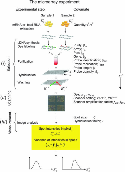
Figure 1.

Illustration of the microarray experiment. The various steps of the experiment and the corresponding covariates used in the model are listed with their symbols. The model consists of three levels: (i) selection, (ii) scanning and (iii) measurement. In (i), $K_g^1$ and $K_g^2$ mRNA molecules for gene g present in sample 1 and 2 undergo a selection process. Each molecule succeeds or fails in each of the experimental steps: cDNA synthesis, dye labelling, purification, hybridization and washing. Success for each molecule is modelled as a Bernoulli coin toss. The success probability depends on properties of the molecule and of the experiment (covariates). Molecules of the same gene can have different covariates, e.g. if they hybridize on different spots with different probes. If probe is in excess, molecules can be modelled as independent variables and the number of remaining molecules after each step is binomially distributed. The probability of successfully passing through the entire experiment is the product of the probabilities of surviving each individual step. Nested binomial variables are binomial and the final number of molecules ready for being scanned is binomial with two parameters: the unknown original number of transcripts per gene in each sample and the selection probability, modelled as in Equation 1. Level (ii) describes the translation of the bound molecules remaining after washing ($H_s^{t,a}$, on array a, spot s, for sample t = 1, 2) into fluorescence intensities, as in Equation 2. Measurement error (iii) of pixel-wise intensities $L_{j,s}^{t,a}$ (on array a, pixel j on spot s for sample t = 1, 2) is assumed to be normally distributed as in Equation 3. This model allows to obtain estimates of absolute concentrations $K_g^1$ and $K_g^2$ together with their posterior marginal probability density, as sketched at the bottom.