Estimation of protein content in wheat samples using NIR hyperspectral imaging and 1D-CNN

Abstract

Wheat protein content is a major determinant of its usage and value. Current methods require wet labs that may be difficult to access and are not real-time. To overcome this, Hyperspectral imaging (HSI) has been reported for estimating the protein content of wheat seeds with the advantage that it is real-time, does not require wet labs, and has high accuracy. However, these models have been developed and validated for a small range of protein content, and without considering cultivation regions. This paper reports the extension of the use of HSI for protein estimation for a wider range of protein content and for wheat cultivated in different regions. Hyperspectral images of 621 wheat samples from five regions in India were acquired in the 900–1700 nm wavelength range. The reference protein content of each sample was determined using the Kjeldahl method, with values ranging from 9.5 to 17.25%. Mean spectra were extracted from the hyperspectral images to develop deep learning and conventional machine learning methods, which were validated through 5-fold cross-validation. The experiments showed that the one-dimensional convolutional neural networks (1D-CNN) performed the best, with the coefficient of determination (R²) of 0.9972, root mean square error (RMSE) of 0.0771, and the ratio of performance to deviation (RPD) of 18.81 for the prediction set. This shows that a 1D-CNN model trained using mean spectra can accurately estimate the wheat protein content. This has the advantage of not requiring a wet lab, and being potentially real-time, which could benefit the farmers, traders, and food industry.

Introduction

Wheat (Triticum spp.) is one of the most widely cultivated cereal crops worldwide. It is a staple food for billions of people and is an important ingredient in livestock feed. The protein concentration in wheat seeds ranges from 9 to 18% of the total kernel weight¹. The difference is due to several factors, such as the variety, weather, and the farm location. The protein content affects the functional properties, flavor, nutritional value, and market price of the seeds. It determines the suitability of wheat for different food products such as pasta, bread, biscuits, and chapatti². Therefore, accurate estimation of the total protein content in wheat seeds is essential.

The traditional methods for determining the wheat protein content are based on the measurement of the amount of nitrogen in the sample. Many chemical and physical approaches are required for sample pre-treatment and often involve the use of toxic reagents. The Kjeldahl method for protein analysis requires approximately 5–6 h per test and consists of three primary steps: digestion, distillation, and titration. The digestion of organic material is achieved using sulfuric acid (H₂SO₄), heat, potassium sulfate (K₂SO₄), and a catalyst. In the distillation step, sodium hydroxide (NaOH) is utilized to release ammonia (NH₃), which is absorbed into a boric acid (H₃BO₃) solution. The nitrogen content is then determined through titration with either hydrochloric acid (HCl) or sulfuric acid (H₂SO₄). This nitrogen content is then used to calculate the protein content of wheat using a conversion factor of 5.7³. These methods are unsuitable in a number of applications where wet labs are not available or the results are required instantaneously⁴.

The absorption of near-infrared (NIR) radiation by the seed sample is indicative of its protein content, and this can offer a fast alternative that does not require a wet lab, making it more suitable for real-time assessments⁵. Hyperspectral imaging (HSI) in NIR region has the advantage of providing the spectrum in the range relevant to protein assessment. A number of different methods have been used for the analysis of the spectrum obtained using HSI to estimate the chemical composition of the seeds^6–8. The methods reported in the literature typically combine spectral analysis with traditional machine learning algorithms such as support vector regression (SVR) or partial least squares regression (PLSR). Caporaso et al.¹ used HSI combined with PLSR to estimate the protein content in wheat, achieving a validation coefficient of determination (R²) of 0.79 and a root mean square error (RMSE) of 0.94. Aulia et al.⁹ coupled HSI with PLSR to predict protein content in soybean seeds, reporting a test R² of 0.92 and an RMSE of 1.08. Cheng et al.¹⁰ employed PLSR to analyze peanut oil and protein content, resulting in R² and RMSE values of 0.945 and 0.196 for oil prediction and 0.901 and 0.441 for protein prediction, respectively. Sun et al.¹¹ explored the use of HSI with the SVR model to assess moisture levels in barley seeds, obtaining a prediction R² of 0.883, an RMSE of 0.0198%, and a ratio of performance to deviation (RPD) of 2.596. These traditional models need pre-processing and feature engineering to interpret the complex hyperspectral datasets effectively. In the field of machine learning, deep learning has emerged as an advanced technique that automatically learns complex patterns and features from hyperspectral data. Singh et al.¹² predicted the protein content of barley seeds from a single growing zone using CNN, achieving R² of 0.9962 and RMSE of 0.0823. Said et al.¹³ employed CNN to estimate the protein content of wheat seeds collected from a single location and achieved the R² of 0.82. Wang et al.¹⁴ employed CNN to predict protein content in 14 wheat varieties, covering a protein range of 9.54%−12.27%, and reported R² of 0.9942 and RMSE of 0.1041. Yuan et al.¹⁵ used camellia seeds from a single variety and origin to predict oil content. They employed a CNN with an attention mechanism, achieving an R² of 0.829 and an RMSE of 2.462. The recent work by Huang et al.¹⁶ used stacked ensemble learning (SEL) to detect the protein content in 14 wheat varieties, which ranged from 9.5 to 14.27, achieving an R² of 0.9939 and an RMSE of 0.0116. However, SEL relies on combining multiple base models, which increases computational complexity and makes it less scalable for larger datasets.

The summary of the review of previous studies indicates that combining NIR-HSI with machine learning has the potential for evaluating seed nutrients. However, previous studies have not tested their models for generalisability by considering the wheat seeds from diverse geographical origins. Another limitation is that these studies have generally considered only a narrow range of protein content. This limits the real-world applications of these models, especially in countries such as India, where wheat is grown in different regions with large climatic and soil conditions, and there is a wide range of protein content in the different cultivated varieties. Therefore, there is a need to develop a model to analyze the spectrum obtained from the HSI that addresses these shortcomings.

This study aimed to explore the feasibility of using the NIR-HSI technique paired with a one-dimensional convolutional neural network (1D-CNN) for estimating wheat protein content across a wide range (9.5–17.25%) in samples collected from five geographical origins. The specific objectives were to: (1) collect hyperspectral images of wheat samples in the spectral range of 900–1700 nm and obtain reference protein content using the Kjeldahl method, (2) extract and preprocess the mean spectra extracted from these samples, (3) evaluate the effectiveness of employing 1D-CNN model for accurate protein content estimation, and (4) compare the performance of 1D-CNN with other deep learning and machine learning models, including SVR, PLSR, and long short-term memory (LSTM).

Methods

Samples preparation

Wheat samples were collected from five distinct geographical locations across three major wheat-growing zones in India: Ludhiana, Karnal, and Jaipur from the North Western Zone; Dharwad from the Peninsular Zone; and Indore from the Central Zone, as shown in Fig. 1. The data collection was carried out during the wheat-harvesting seasons of 2021 and 2022. Comprehensive details regarding the wheat varieties used are provided in Table 1. A total of 621 wheat samples were used, with each sample weighing approximately 15 g. The seeds were stored in airtight containers and refrigerated at 4 °C to preserve their quality¹². Prior to data acquisition, the samples were taken out at a temperature of 262 °C and a relative humidity of 552% for twelve hours. Moisture content was determined using the oven drying method (ISO 712:2009), yielding a moisture range of 11–12.5% (wet basis). As shown in Fig. 2(a), the wheat samples were arranged on a tray specifically designed for hyperspectral data acquisition. The tray was coated with black paint to reduce undesired reflections. After the data acquisition process, the protein content of each sample was determined using the Kjeldahl method¹⁴.

Fig. 1.

Map showing the locations across India from which wheat samples were collected.

Table 1.

Details of wheat samples collected from different zones and locations across india, listing the specific varieties and their respective counts.

Zone	Location	Variety name	Counts
North Western	Ludhiana	DBW187, DBW222, HD3086, PBW1Zn, PBW343U, PBW550U, PBW590, PBW658, PBW677, PBW725, PBW771, PBW803, PBW826, PBW833, PBW835, PBW869, PDW291, WH1105	18
	Karnal	A9-30-1, BIJAGAR, C306, DBW107, DBW110, DBW168, DBW173, DBW17, DBW252, DBW88, DDK1001, DDK1009, DDK1025, DDK1029, DDW47, DPW621-50, DT46, GW1139, GW322, HD2733, HD2967, HD3226, HI8498, HW1098, MACS2694, MACS2971, MP3465, NP200, PBW343, PBW373, PBW502, PBW752, PDW274, TL2908, TL2942, WB2, WH1184	37
	Jaipur	CCNRV1, RAJ1482, RAJ3077, RAJ3765, RAJ3777, RAJ4037, RAJ4079, RAJ4083, RAJ4120, RAJ4238	10
Central	Indore	HD4728, HI1605, HI1634, HI1636, HI8663, HI8713, HI8737, HI8759, HI8777, HI8823	10
Peninsular	Dharward	MACS3949, MACS4100, UAS304, UAS334, UAS347, UAS375, UAS428, UAS446	8

Fig. 2.

The steps involved in hyperspectral image processing and extraction of multiple mean spectra.

Hyperspectral camera specifications and image correction

A reflection mode pushbroom HSI camera was employed to capture hyperspectral images of wheat samples (Fig. 2(b)). The experimental setup comprised a spectrograph, a 14-bit Indium Gallium Arsenide (InGaAs) camera, four 35 W coherent halogen bulbs, a translation stage, and a computer that supports hypercube acquisition software (SpectrononPro 2.96). The hyperspectral camera utilized in this study operates on a line-scanning mechanism, capturing 320 pixels per line with 164 spectral bands. The spectrograph integrated into the camera covers a spectral range of 900–1700 nm, providing a spectral resolution of 4.9 nm. The halogen bulbs were positioned in a ring configuration at an approximately 45-degree angle and around 250 mm above the translation stage for uniform and continuous illumination of samples. The entire arrangement was enclosed within a custom-made dark chamber to maintain controlled lighting conditions throughout the image acquisition process. To ensure accurate data collection and prevent distortion in the hypercube, the camera settings were optimized with a frame rate of 41 Hz, an integration time of 2.16 ms, and a translation stage speed of 14.22 mm/s. To ensure stability, the camera and light source were turned on 30 min before image acquisition. The dimensions of the captured hypercube have a resolution of 320 × 850 × 164 (x × y × λ), where the spatial and spectral dimensions are represented along the x, y, and λ (spectral bands) axes, respectively. Following image acquisition, image correction was performed by capturing white and dark reference images. Black and white correction is a fundamental step to reduce the influence of dark current and uneven light sources and normalize pixel values as reflectance values¹⁷. The dark reference was obtained by covering the lens aperture completely, while a white reference was captured using a standard white Fluorilon tile. After image correction, the spectral dimensions of the hypercube were refined by excluding the first 14 bands and the last 7 bands, resulting in a spectral range of 955.62 to 1688.87 nm, comprising 147 distinct wavelengths.

Hyperspectral data pre-processing and spectral data extraction

The hyperspectral images of the wheat samples were processed using a 3 × 3 median filter to enhance data quality by removing the presence of any dead pixels from the hypercube¹⁸. Subsequently, binary thresholding was applied to separate the wheat samples from the tray¹⁹. For this purpose, the image at the spectral band of 1088.1 nm was selected due to a clear distinction between the pixels of the wheat sample and the tray (Fig. 2(c)). A threshold value of 0.19 was applied to the selected image, resulting in a binary mask (see Fig. 2(d)). This binary mask (Fig. 2(e)) was then used across all wavelengths to select a region of interest (ROI) (see Fig. 2(f)). All these operations were performed using the Python OpenCV and Scikit-image Library.

There are two primary approaches to extracting the spectral data from the ROIs: pixel-wise and sample-wise spectrum²⁰. Pixel-wise spectrum is obtained using the reflectance values of a pixel across all the wavelengths. Figure 2(g) displays the pixel-wise spectra, where each grey curve represents the spectrum for individual pixels within the ROI. The variability among these spectra is due to the inherent heterogeneity of the pixel-level reflectance values and the scattering effects caused by the physical attributes of the seeds, including their shape and surface curvature. On the other hand, the sample-wise spectrum is calculated by averaging all pixel-wise spectra, as represented by the black curve in Fig. 2(h). This approach allows for the extraction of representative spectral signatures at the sample level, effectively reducing the noise and variability introduced by the individual pixel-wise spectrum²⁰.

In this study, we obtained the multiple mean spectra from a sample by averaging randomly selected subsets of pixel-wise spectra. A total of 90 mean spectra were derived, as illustrated by the red curves in Fig. 2(h). Extracting multiple mean spectra offers several advantages over both pixel-wise and sample-wise approaches. Compared to pixel-wise spectra, this method reduces noise by averaging subsets of pixels, resulting in more robust spectral representations. Furthermore, unlike the single sample-wise spectrum, this approach generates multiple representative spectra per sample, effectively augmenting the data. This is particularly beneficial in scenarios with limited samples, where determining ground truth through chemical methods is expensive and time-consuming.

After extracting the spectral data, several pre-processing methods were applied to reduce the effects related to light scattering caused by sample morphology²¹. Selecting an appropriate spectral preprocessing technique is challenging due to the absence of standardized guidelines, making it difficult to generalize methods²². Therefore, we compared different preprocessing techniques, including Savitzky-Golay smoothing (SGS), SG first derivative (SG1) and SG second derivative (SG2), standard normal variate (SNV), multiplicative scatter correction (MSC), and detrending, to identify the most suitable method for our analysis. The spectral data was pretreated using the Python packages Scikit-learn and SciPy, which provide functions and modules for implementing these preprocessing techniques.

Regression models

The wheat protein content was predicted using two traditional models and two deep learning regression models, PLSR, SVR, LSTM, and 1D-CNN. These methods are widely used in spectral data analysis for their distinct computational principles and their ability to effectively capture the relationships between spectral features and chemical properties^23,24.

PLSR is a widely adopted linear regression technique that projects the input spectral data and target protein values into a latent space and maximizes their covariance²⁵. The number of latent variables, which is a crucial parameter affecting the model’s performance, was optimized within the range of 2 to 40 using 5-fold cross-validation. SVR is a nonlinear regression method that predicts the target values by finding a function within a margin of tolerance. The input features are mapped into a higher-dimensional space using kernel functions to capture complex relationships between spectral features and protein values²⁶. In this study, the radial basis function (RBF) kernel was employed, and model parameters, including the kernel width (γ) and penalty parameter (C), were fine-tuned using a grid search combined with 5-fold cross-validation. The search range for γ and C was systematically varied from 2⁻⁷- 2⁷. Both the traditional models were implemented using the Python Scikit-learn Library.

LSTM, a type of recurrent neural network, is well-suited for sequential data tasks due to its ability to capture long-term dependencies²³. The LSTM architecture consists of input, forget, and output gates, along with memory cells, to address the vanishing gradient problem. Likewise, 1D-CNN is widely recognized as one of the most advanced techniques for analyzing spectral data. It enables the extraction of intricate and meaningful features within the spectral data by using its deep and multi-layered architecture⁶. The optimal hyperparameters for both LSTM and 1D-CNN models were selected using a grid search approach. Batch normalization and dropout were used to improve the model’s training stability and prevent overfitting. The Adam optimizer was employed to train the model, with mean squared error (MSE) serving as the loss function. In this study, the LSTM architecture was designed with two LSTM blocks followed by three fully connected (FC) layers. A dropout layer with a rate of 0.3 was added before the FC layers, and the model was trained using backpropagation through time (BPTT) with a learning rate of 0.0001. The optimal hyperparameters and the proposed architecture of the 1D-CNN model are presented in Table 2; Fig. 3, respectively. Both deep learning models were implemented using TensorFlow and trained on an 8 GB NVIDIA Quadro RTX 4000 graphics processing unit. The entire methodology was executed using an Intel Xeon processor with 96 GB of RAM.

Table 2.

Optimal hyperparameters of the 1D-CNN model.

Optimal hyperparameter	Value
Number of convolutional layers	2
Number of fully connected layers	5
Number of filters	[32, 64]
Filter size	9
Drop out in convolutional and FC layers	0.2
Drop out after flattening layer	0.5
Activation Function	Leaky ReLU
Learning rate	0.0001
Batch Size	32
Number of epochs	300

Fig. 3.

Architecture of the proposed 1D-CNN model for wheat protein estimation.

Model evaluation and validation

The dataset comprised 621 wheat samples, which were randomly split into a training set of 496 samples (80%) and a testing set of 125 samples (20%). This splitting ratio provides sufficient data for model training while ensuring a portion remains available for performance evaluation. The 80 − 20 partitioning of data has been widely adopted in previous studies, demonstrating its effectiveness in developing stable and reliable models^12,27. A 5-fold cross-validation was applied to these 496 samples to select the optimal hyperparameters for the models, identify the most effective spectral preprocessing techniques, and minimize the risk of overfitting.

The regression models used in this study were evaluated using three key metrics: R², RMSE, and RPD. These metrics compare the predicted protein content to the actual values, providing insights into the models’ predictive accuracy. R² measures how well the predicted protein content aligns with the reference values. It ranges from 0 to 1, where higher values indicate stronger predictive accuracy. RMSE quantifies the average error between predicted and actual values, with lower RMSE indicating a more precise model. RPD evaluates the model’s predictive ability to the inherent variability in the reference data. It is calculated as the ratio of the standard deviation of reference protein values to the RMSE. An RPD value above 8 suggests excellent predictive performance²⁸. The formulas and detailed explanations of these metrics are available in Singh et al.¹². All these metrics were computed using the Python Scikit-learn library.

Results and discussion

Spectral visualization and statistical analysis of reference values

The average reflectance spectral curves for 621 wheat samples within the wavelength range of 900 to 1700 nm are illustrated in Fig. 4. The spectral curves of samples having different protein content visually appear to have a consistent overall shape, with peaks and valleys occurring at similar wavelengths. There appear to be three absorption peaks, which are located around 980 nm, 1200 nm, and 1450 nm, as shown with black arrows in Fig. 4. The peak near 980 nm is linked to moisture content, representing the second overtone of the O-H bond. The absorption at 1200 nm is broader, indicating the presence of carbohydrates, and is attributed to the second overtone of the CH bond. The wide absorption band at 1450 nm is associated with both protein and moisture, corresponding to the first overtones of the NH and OH bonds, respectively¹⁸. While having similar shapes of the spectrum, there are differences in the reflectance values, which, however, may be due to differences in the samples or other factors, such as differences in incident light due to the shape of the seed. With possibly subtle differences in the spectrum of seeds with different protein content, one option is to use machine or deep learning techniques to estimate the protein content of different wheat samples.

Fig. 4.

The spectral characteristics of wheat samples used in this study.

The statistical analysis of protein content (%) measured using a Kjeldahl method is summarized in Table 3. The dataset comprised 621 samples, with a mean protein content of 12.45% and a standard deviation (SD) of 1.42%. Protein values ranged from 9.5 to 17.25%. The dataset was randomly divided into training and testing sets to develop and evaluate the predictive models, with 80% of the data allocated for training and 20% for testing. The training set included 496 samples with a mean of 12.45% and an SD of 1.41%, while the testing set comprised 125 samples with a mean of 12.45% and an SD of 1.45%.

Table 3.

The statistics of wheat protein content (%) measured using the Kjeldahl method.

Sample set	N *	MeanSD	Minimum	Maximum
Training set	496	12.451.41	9.5	17.25
Testing set	125	12.451.45	9.5	17.25
Total	621	12.451.42	9.5	17.25

^*Number of samples

Protein estimation using 1D-CNN

This study implemented a 1D-CNN to estimate protein content in wheat seeds using spectral data. The 496 training samples were subjected to 5-fold cross-validation to ensure robust model performance by selecting optimal hyperparameters and reducing the risk of overfitting. Multiple mean spectra were obtained from the samples to improve the model’s performance. Specifically, 90 mean spectra were generated for each sample in the training and validation sets, resulting in a total of 35,640 spectra for training and 9,000 spectra for validation. These spectra served as input to train the 1D-CNN model. Different hyperparameter configurations were assessed during the training process, as depicted in Fig. 5. The impact of these hyperparameters on the model’s performance was evaluated by calculating the mean and standard deviation of R² and RMSE values across five splits of 5-fold cross-validation. Each bar represents the mean value for the metric, accompanied by error bars indicating the standard deviation. The optimized 1D-CNN model achieved a high R² of 0.99250.0007 and RMSE of 0.12150.0052 on the training set. For the validation set, the model attained an R² of 0.98740.0024 and an RMSE of 0.16350.0101. It can also be observed from Fig. 5 that the inclusion of pooling layers in the model resulted in a reduction in accuracy, which may be attributed to the loss of spectral information. Figure 6 presents the loss versus epoch curves for the models over 300 training epochs. An epoch refers to one complete pass through the entire training dataset during the learning process. Multiple epochs are typically required to allow the model to gradually minimize error and improve its predictive performance²⁹. As shown in the figure, the 1D-CNN model exhibited a rapid decrease in loss during the initial epochs, followed by a saturation, indicating that the model converged toward optimal performance within 300 epochs.

Fig. 5.

Performance evaluation of the 1D-CNN model with different hyperparameters.

Fig. 6.

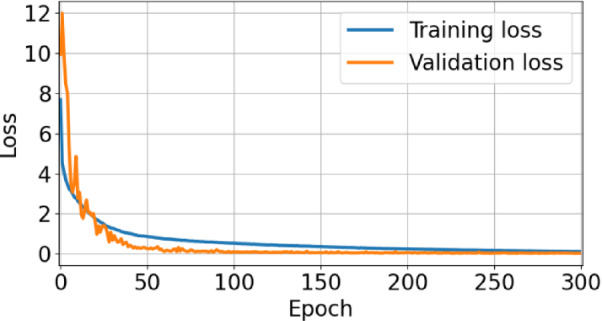
Training and validation loss curves of the 1D-CNN model over 300 epochs.

Figure 7 shows the spectral signatures of the dataset after applying six preprocessing techniques. Each preprocessing method addresses different issues in raw spectral data. For example, SNV and MSC reduce scatter effects and normalize spectral intensity, SGS smooths the spectra, SG1 and SG2 enhance sharp spectral features by calculating first and second derivatives, emphasizing subtle changes in the data, detrending removes baseline variations, improving the clarity of absorbance or reflectance peaks²¹. Figure 8 illustrates the performance of the 1D-CNN model with each of the six preprocessing techniques evaluated on the validation set. The left bar graph shows the R² values, whereas the right bar graph represents the RMSE values. The highest R² value of 0.98740.0024 and lowest RMSE of 0.1635 0.0101 was achieved with the raw data, indicating strong predictive performance without preprocessing. The filters in the convolutional layers in 1D-CNN act as an automatic pre-processor that could extract effective information from raw spectra²⁹. Other methods, such as SGS, SG1, SG2, SNV, Detrend, and MSC, had slightly lower performance, reflecting that these techniques may be filtering out the features that are relevant to the protein content. The results demonstrate that the 1D-CNN model is effective for predicting protein content from spectral data without preprocessing requirements.

Fig. 7.

Spectral signatures after applying various preprocessing techniques: (a) SNV, (b) MSC, (c) SGS, (d) SG1, (e) SG2, and (f) detrending.

Fig. 8.

Impact of spectral preprocessing techniques on 1D-CNN model performance.

Comparison of regression models

The performance (mean standard deviation) metrics of the four regression models, 1D-CNN, LSTM, SVR, and PLSR, are presented in Table 4. The results show that the 1D-CNN model, trained on raw spectral data, achieved the highest R² of 0.9874, the lowest RMSE of 0.1635, and the highest RPD of 9.03. Following the 1D-CNN model was LSTM with R² of 0.9363 and an RMSE of 0.2883. The SVR showed lower accuracy compared to both 1D-CNN and LSTM, with an R² of 0.9086 and an RMSE of 0.5335. The PLSR model had the lowest performance with an R² of 0.5955 and the highest RMSE of 1.4046. Overall, the results show that the 1D-CNN model outperformed other applied models for protein assessment with minimal error.

Table 4.

Performance comparison of the 1D-CNN model with LSTM, PLSR, and SVR models on the validation set.

Model	Spectral preprocessing	Hyperparameters*	n **		RMSE	RPD
1D-CNN	Raw data	(300, 32, 11)	90	0.98740.0024	0.16350.0101	9.03.83
LSTM	SG2	(400, 64)	70	0.93630.0231	0.28830.0612	4.810.58
SVR	SG2	(8, 0.03125)	30	0.90860.0766	0.53350.0586	3.610.76
PLSR	Detrending	21	40	0.59550.0499	1.40460.0383	1.590.13

^*Hyperparameters: (batch size, epochs, filter size) for 1D-CNN model, (epochs, batch size) for LSTM, (C, γ) for SVR model, latent variables for PLSR model.

^**n: number of mean spectra.

Performance evaluation of the 1D-CNN model

The 1D-CNN model was evaluated using 20% of the dataset that was not used during the training. Figure 9 shows the scatter plot of the correlation between predicted and actual protein content. The model achieved performance with an R² value of 0.9972, an RMSE of 0.0771, and an RPD of 18.81. The results in the mix of regions and the large protein content range show the model’s suitability for practical applications in industries requiring precise protein quantification without a wet lab.

Fig. 9.

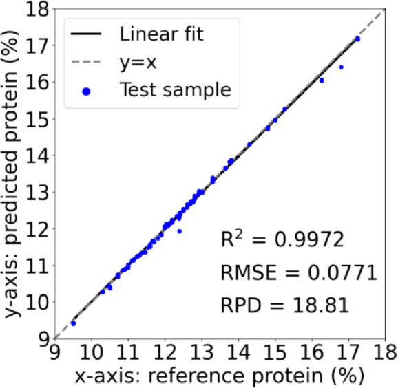
Scatter plot showing the correlation between predicted and actual wheat protein content.

To assess the significance of extracting multiple mean spectra, we evaluated the performance of the 1D-CNN model based on the number of mean spectra obtained per sample. Figure 10 illustrates that the predictive power of the 1D-CNN model depended on the number of mean spectra used. When only one spectrum per sample was included, the highest RMSE value of 3.2397 was observed, indicating poor predictive accuracy due to undertraining. However, as the number of mean spectra per sample increased, the RMSE value decreased, reaching a minimum of 0.0771 at n = 90, suggesting an optimal balance for representing the spectral information of the samples. Beyond this point, further increasing the number of mean spectra led to a rise in RMSE, likely due to variability between the mean spectra and the actual sample spectra. Overall, using 90 mean spectra per sample was identified as the optimal choice for enhancing the 1D-CNN model’s predictive performance.

Fig. 10.

Impact of the mean spectra count on the RMSE performance of the 1D-CNN model.

Innovations

This study reports an accurate HSI-based technique for the estimation of protein content in wheat seeds, with R²0.9972, RMSE0.00771, and RPD18.81. When compared to other similar studies, our model represents a wider range of protein content, from 9.5 to 17.25% by weight, indicating its generalizability. Another highlight of this work is that it is built on wheat cultivation from five regions covering different climatic conditions, further showing that this model is generalizable. The outcome of this work is a model that has the potential to be used to estimate the protein content in the wheat samples without requiring a wet lab and thus could be used in real-world applications during the commercial trading of wheat.

Limitations and future work

This study has three major limitations. The first is that while this method does not require a wet lab, however, it requires a specially built chamber for hyperspectral imaging, which is not portable and inexpensive. There is a need to transfer these findings to develop a low-cost, portable device. Another limitation is that the wheat samples were limited to five regions of India and did not include wheat samples from other regions. There is a need to test this model for other regions around the world. Lastly, the current study focuses on a single-task 1D-CNN model for protein prediction, which restricts its ability to simultaneously analyze multiple seed quality parameters.

Conclusion

Accurate protein content estimation in wheat samples is crucial for the food industry and agricultural sectors to ensure nutritional standards and crop quality. This study demonstrated the feasibility of using near-infrared hyperspectral imaging (NIR-HSI) combined with a one-dimensional convolutional neural network (1D-CNN) for accurately estimating wheat protein content. Wheat samples were collected from five different geographical origins in India, and their reference protein content, measured using the Kjeldahl method, exhibited a broad range from 9.5 to 17.25%. The spectral information in the 900–1700 nm range was extracted from the hyperspectral images of wheat samples, and preprocessing techniques were employed. The convolutional filters within the 1D-CNN model functioned as an automatic preprocessor, efficiently extracting meaningful spectral features directly from raw data without the need for spectral preprocessing. The proposed 1D-CNN model outperformed other models, including SVR, PLSR, and LSTM, with an R² of 0.9972, an RMSE of 0.0771, and an RPD of 18.81. These results confirm that spectral data derived from hyperspectral images of wheat samples were sufficient to build highly accurate models for protein estimation. The inclusion of a wide protein range and diverse geographical origins further enhances the robustness and generalizability of the model, indicating its potential applicability across varied wheat-growing conditions. These findings indicate the potential of using HSI in the NIR range combined with 1D-CNN for real-time estimation of protein content in wheat samples without the use of a wet lab. However, further work is required for these findings to make a portable and inexpensive device.

Author contributions

Apurva Sharma: Conceptualization, design of experiments, data collection, implementation, interpretation of results, drafted the manuscript; Tarandeep Singh: assisted in the experimental setup, data collection, contributed to model development and analysis; Neerja Garg and Dinesh Kumar: resources, supervision, manuscript editing and revision; Quoc Cuong Ngo: supervision and manuscript revision.

Data availability

The dataset used in this study will be made available upon a reasonable request. Please contact Neerja Mittal Garg at neerjamittal@csio.res.in for access to the data.

Declarations

Competing interests

The authors declare no competing interests.

References

- 1.Caporaso, N., Whitworth, M. B. & Fisk, I. D. Protein content prediction in single wheat kernels using hyperspectral imaging. Food Chem.240, 32–42 (2018). [DOI] [PMC free article] [PubMed] [Google Scholar]
- 2.Shuqin, Y., Dongjian, H. & Jifeng, N. Predicting wheat kernels ’ protein content by near infrared hyperspectral imaging. International Journal of Agricultural and Biological Engineering.9, 163–170 (2016).
- 3.Safdar, L. B. et al. Reviving grain quality in wheat through non-destructive phenotyping techniques like hyperspectral imaging. Food Energy Secur.12, 1–21 (2023). [DOI] [PMC free article] [PubMed] [Google Scholar]
- 4.Shi, T. et al. Using VIS-NIR hyperspectral imaging and deep learning for non-destructive high-throughput quantification and visualization of nutrients in wheat grains. Food Chem.461, 140651 (2024). [DOI] [PubMed] [Google Scholar]
- 5.Wang, B. et al. The applications of hyperspectral imaging technology for agricultural products quality analysis: A review. Food Rev. Int.39, 1043–1062 (2023). [Google Scholar]
- 6.Dhanya, V. G. et al. High throughput phenotyping using hyperspectral imaging for seed quality assurance coupled with machine learning methods: principles and way forward. Plant. Physiol. Rep.29, 749–768 (2024). [Google Scholar]
- 7.Wu, K. et al. Using visible and NIR hyperspectral imaging and machine learning for nondestructive detection of nutrient contents in sorghum. Scientific Reports, 15(1), 6067 (2025). [DOI] [PMC free article] [PubMed]
- 8.Hamad, R. & Chakraborty, S. K. A chemometric approach to assess the oil composition and content of microwave-treated mustard (Brassica juncea) seeds using Vis–NIR–SWIR hyperspectral imaging. Sci. Rep.14, 1–13 (2024). [DOI] [PMC free article] [PubMed] [Google Scholar]
- 9.Aulia, R. et al. Non-destructive prediction of protein contents of soybean seeds using near-infrared hyperspectral imaging. Infrared Phys. Technol.127, 104365 (2022). [Google Scholar]
- 10.Cheng, J. H., Jin, H., Xu, Z. & Zheng, F. NIR hyperspectral imaging with multivariate analysis for measurement of oil and protein contents in peanut varieties. Anal. Methods. 9, 6148–6154 (2017). [Google Scholar]
- 11.Sun, H., Zhang, L., Rao, Z. & Ji, H. Determination of moisture content in barley seeds based on hyperspectral imaging technology. Spectrosc. Lett.53, 751–762 (2020). [Google Scholar]
- 12.Singh, T., Garg, N. M., Iyengar, S. R. S. & Singh, V. Near-infrared hyperspectral imaging for determination of protein content in barley samples using convolutional neural network. J. Food Meas. Charact.10.1007/s11694-023-01892-x (2023). [Google Scholar]
- 13.Said, I. et al. Seed protein content Estimation with Bench-Top hyperspectral imaging and attentive convolutional neural network models. Sensors.25, 303 (2025). [DOI] [PMC free article] [PubMed]
- 14.Wang, J. et al. Rapid detection of protein and starch content in brewing wheat using hyperspectral imaging technology combined with a convolutional neural network regression model. J. Am. Soc. Brew. Chem.82, 323–334 (2024). [Google Scholar]
- 15.Yuan, W. et al. Prediction of oil content in camellia Oleifera seeds based on deep learning and hyperspectral imaging. Ind. Crops Prod.222, 119662 (2024). [Google Scholar]
- 16.Huang, Y., Tian, J., Yang, H., Hu, X. & Han, L. Detection of wheat Sacchari Fi cation power and protein content using stacked models integrated with hyperspectral imaging. (2024). 10.1002/jsfa.13296 [DOI] [PubMed]
- 17.Peng, J. et al. Determination of malathion content in sorghum grains using hyperspectral imaging technology combined with stacked machine learning models. J. Food Compos. Anal.135, 106635 (2024). [Google Scholar]
- 18.Sharma, A., Singh, T. & Garg, N. M. Nondestructive identification of wheat seed variety and geographical origin using Near-Infrared hyperspectral imagery and deep learning. J. Chemom. 38, 1–12 (2024). [Google Scholar]
- 19.Singh, T., Garg, N. M. & Iyengar, S. R. S. Nondestructive identification of barley seeds variety using near-infrared hyperspectral imaging coupled with convolutional neural network. Journal of Food Process Engineering vol. 44Springer International Publishing, (2021).
- 20.Zhang, C., Liu, F. & He, Y. Identification of coffee bean varieties using hyperspectral imaging: influence of preprocessing methods and pixel-wise spectra analysis. Sci. Rep.8, 1–11 (2018). [DOI] [PMC free article] [PubMed] [Google Scholar]
- 21.Dai, Q. et al. Recent advances in De-Noising methods and their applications in hyperspectral image processing for the food industry. Compr. Rev. Food Sci. Food Saf.13, 1207–1218 (2014). [Google Scholar]
- 22.Saha, D., Senthilkumar, T., Sharma, S., Singh, C. B. & Manickavasagan, A. Application of near-infrared hyperspectral imaging coupled with chemometrics for rapid and non-destructive prediction of protein content in single Chickpea seed. J. Food Compos. Anal.115, 104938 (2023). [Google Scholar]
- 23.Pang, L. et al. Feasibility study on identifying seed viability of sophora Japonica with optimized deep neural network and hyperspectral imaging. Comput Electron. Agric190, 106426 (2021).
- 24.Xu, M. et al. Non-destructive Estimation for Kyoho grape shelf-life using vis/nir hyperspectral imaging and deep learning algorithm. Infrared Phys. Technol.142, 105532 (2024). [Google Scholar]
- 25.Mulowayi, A. M. et al. Quantitative measurement of internal quality of carrots using hyperspectral imaging and multivariate analysis. Sci. Rep.14, 1–14 (2024). [DOI] [PMC free article] [PubMed] [Google Scholar]
- 26.Chu, B. et al. Nondestructive determination and visualization of protein and carbohydrate concentration of chlorella pyrenoidosa in situ using hyperspectral imaging technique. Comput. Electron. Agric.206, 107684 (2023). [Google Scholar]
- 27.Varrà, M. O., Ghidini, S., Ianieri, A. & Zanardi, E. Near infrared spectral fingerprinting: A tool against origin-related fraud in the sector of processed anchovies. Food Control123, 107778 (2021).
- 28.Manley, M. Near-infrared spectroscopy and hyperspectral imaging: Non-destructive analysis of biological materials. Chem. Soc. Rev.43, 8200–8214 (2014). [DOI] [PubMed] [Google Scholar]
- 29.Cui, C. & Fearn, T. Modern practical convolutional neural networks for multivariate regression: applications to NIR calibration. Chemom Intell. Lab. Syst.182, 9–20 (2018). [Google Scholar]
Associated Data
This section collects any data citations, data availability statements, or supplementary materials included in this article.
Data Availability Statement