A simulation of thermal coupling characteristics on deep-sea residual oil recovery via pipeline using thermophysical properties

Abstract

Deep-sea residual oil has been recognized as a significant environmental hazard due to its poor low-temperature fluidity and complex recovery processes necessitating urgent solutions. A segmented regulated two stage heating transport method is proposed, with a high-precision thermo-fluid coupling model that integrates thermophysical properties to characterize oil thermal coupling characteristics. Dimensional analysis further identifies multi-properties correlations for convective heat transfer coefficient and oil temperature that govern the thermo-fluid dynamics interaction. Numerical simulations reveal that transport distance, heat flux density, and mass flux collectively regulate convective heat transfer efficiency and temperature distribution. It is shown that oil temperatures reduce oil viscosity, thereby enhancing convective heat transfer between the thermal boundary layer oil and the pipe wall; as transport distance increases, accumulated heat and thermophysical properties stabilize simultaneously. A dual-properties regulation mechanism is identified between heat flux density and mass flux: within 180–540 kg/(m²·s), outlet thermal boundary layer oil temperature linearly responds to heat flux density (K = 0.04); exceeding 720 kg/(m²·s), temperature regulation efficiency decreases by 30%, accompanied by a downstream shift of temperature peak region under high mass flux conditions. This method provides reliable theoretical foundations for deep-sea low-temperature residual oil recovery.

Introduction

Significant accumulation of residual oil in deep-sea environments was caused by an increase in shipwrecks and underwater accidents in recent years. The efficient recoveries of oil were deemed critical to mitigate marine ecological pollution and reduce hydrocarbon leakage risks, addressing a strategic imperative^1–4. As shown Fig. 1, Under deep-sea conditions, oil viscosity was increased and flowability was reduced by extremely low-temperatures, thereby rendering conventional recovery methods ineffective. Thus, oil viscosity reduction and recovery efficiency improvement were achieved through heating pipeline during recovery operations. The thermal behavior of high-viscosity oil in heated pipeline under deep-sea low-temperature conditions was investigated, offering essential technical insights for developing targeted recovery strategies. Such investigations also contributed theoretically to advancing understanding of fluid transport in complex hydrodynamic systems.

Fig. 1.

Current status of deep-sea oil recovery.

Recent experimental studies revealed that oil exhibits pronounced temperature-dependent viscosity-temperature characteristics, with dynamic viscosity showing far greater temperature sensitivity than thermal properties such as specific heat capacity, density, and thermal conductivity. Zhao et al.⁵ experimentally demonstrated that heavy oil’s dynamic viscosity was 20 times higher than medium crude oil, whereas density and other physical properties exhibited minimal variation. This underscores viscosity-temperature behavior as the thermophysical factor in heavy oil transport. Huerta F et al.⁶ further validated this finding through systematic analysis of phase property dynamics, confirming viscosity parameters display significantly greater temperature responsiveness than other thermophysical indices. Follow-up studies combined multiscale experiments and numerical simulations to systematically investigate rheological structure-property relationships between high-viscosity oil and asphalt components. These studies identified temperature-sensitive viscosity parameters as key constraints for low-temperature pipeline design^7–10. Consequently, temperature-dependent viscosity behavior was recognized as a critical thermophysical constraint necessitating prioritization in heavy oil pipeline design. Precise characterization of this parameter remains indispensable for optimizing transport protocols.

Due to the high complexity of system models, previous research has primarily relied on theoretical methodologies. Those studies employed finite element analysis (FEA) and computational fluid dynamics (CFD) to quantitatively analyze thermal distribution and flow characteristics^11–18. Mostafa M.Abdelhafiz et al.¹⁹ systematically employed CFD techniques to investigate flow-regime-dependent thermal distribution patterns in pipeline systems. Their work numerically solved heat transfer governing equations and integrated convective heat transfer coefficient (CHTC) formulas applicable to both laminar and turbulent flows, revealing an inverse relationship between fluid dynamics properties and temperature distribution under varying flow regimes. Sánchez et al.²⁰ developed a Multiphysics-coupling framework to analyze environmental thermal effects on oil’s hydrodynamic behavior. This framework utilized hybrid numerical schemes and analytical approximations to effectively solve coupled flow-thermal field equations, providing theoretical foundations for thermophysical responses under complex operating conditions. Xu et al.²¹ combined experimental methods with CFD to quantitatively investigate oil’s thermal conduction behavior in pipeline systems. Their innovation involved developing a 3D thermo-fluid coupling model that integrated natural convection effects and temperature-dependent thermal resistance. By thermal influence zone geometry’s regulatory role on temperature fields, this model provided a numerical validation framework for thermal management strategies in complex pipeline networks. Xie et al.²² established a 3D thermal conduction FEA model for pipeline systems, quantitatively revealing the regulatory mechanism of oil’s micro-phase changes on thermophysical responses. Collectively, these studies demonstrated that thermo-fluid coupling modeling is the cornerstone method for oil pipeline systems’ thermophysical behaviors^23–26. However, model accuracy and engineering applicability require further optimization to address complex operational scenarios.

While advancements in quantitative studies of thermo-fluid coupling behavior have been achieved via analytical and numerical methods in recent years, the role of temperature-dependent thermophysical properties in heat transfer mechanisms and the multiparameter coupling effects of operational and geometrical parameters on oil thermal behavior in high-temperature pipeline remain underexplored. To address these gaps, a two-stage segmented heating strategy was proposed for deep-sea oil recovery. This strategy combines preheating oil from low-temperature condensation to a micro-flow state at 20 ℃with continuous convective heat exchange through electrically heating pipeline, thereby mitigating challenges such as poor fluidity and inefficient thermal management during low-temperature transport. Consequently, this approach improves fluid conveyance efficiency and reduces recovery time. A high-precision thermophysical properties correlation model is employed to systematically analyze temperature-dependent nonlinear variations in oil viscosity, density, and specific heat capacity. Additionally, a multiparameter coupling model is developed via dimensional analysis to clarify relationships between convective heat transfer coefficients, thermal boundary layer oil temperatures, and thermophysical parameters (viscosity, density, specific heat capacity, thermal conductivity), flow parameters (velocity), geometrical parameters (transport distance, pipeline diameter). Numerical simulations further demonstrate that transport distance, heat flux density, and mass flux dominantly influence the dynamic equilibrium of thermo-fluid coupling processes by modulating convective heat transfer efficiency, temperature fields gradient distributions, and flow regimes. This work provides a theoretical framework for multi-physics coupling simulations and establishes a basis for optimizing energy efficiency and reliability in deep-sea low-temperature oil heating transport systems. The findings also offer practical insights to enhance safety and energy efficiency in marine residual oil recovery.

Model development methods

Thermal properties parameters of residual oil

Before establishing the mathematical model for the heated transport of low-temperature high-viscosity oil pipelines, it is necessary to clarify the temperature dependence of each thermophysical parameter. As shown in Fig. 2a, the viscosity of oil decreases rapidly with the increase of temperature. When the temperature reaches the wax precipitation point of 46 ℃²⁷, the first derivative discontinuity occurs in the viscosity-temperature characteristic curve, marking the critical interval for the system to transition from a non-Newtonian fluid state to a Newtonian fluid state, presenting semi-flow characteristics. When the temperature continues to rise to 65 ℃, the viscosity drops to 30.55 mPa·s. At this time, the paraffin particles in the oil are completely dissolved, the system is transformed into a Newtonian fluid, the intermolecular force is significantly weakened, and the viscosity is insensitive to temperature. The viscosity-temperature characteristic formula of oil obtained by fitting experimental data can be expressed as:

1

Fig. 2.

Thermal properties of oil as a function of temperature:(a) Viscosity. (b) Density and Specific heat capacity.

where t_f is the temperature of oil (℃), and µ_f is the viscosity of oil (mPa·s).

With the increase of temperature, the kinetic energy of oil molecules is significantly enhanced, leading to the expansion of the average distance between molecules and triggering the volume expansion effect. As shown in Fig. 2b, the density of oil shows a monotonically decreasing trend with the increase of temperature, and its variation law can be described by the density-temperature relationship:

2

where ρ_f is the density of oil (kg/m³).

The specific heat capacity of oil exhibits a turning trend of first decreasing and then increasing with temperature. Thermophysical analysis indicates that when the temperature rises to the wax precipitation point (46 ℃), solid wax crystals start to dissolve, leading to a phase transition of the system. As the temperature further increases above 65 ℃, the thermal motion freedom of liquid wax molecules increases, and the heat required to maintain the temperature rise significantly increases, causing a characteristic inflection point in the specific heat capacity of the system after the wax precipitation point (as shown in Fig. 2b). The relationship between specific heat capacity and temperature can be described by the following equation:

3

where C_p is the specific heat capacity of oil (kJ/(kg·℃)).

Based on the thermal conductivity prediction methodology established by F. Ramos-Pallares²⁸, which accounts for distillate properties, asphaltene content, molecular weight, and fluid specific gravity, the thermal conductivity exhibits dependence on both temperature and density. Below the temperature threshold of 45 ℃, the thermal conductivity is measured at 0.25 W/(m·℃), attributed to the formation of an ordered crystalline lattice structure facilitating efficient phonon-mediated heat transfer. Above 45 ℃, the thermal conductivity decreases to 0.15 W/(m·℃) due to the disintegration of the crystalline framework. This phase transition induces a disordered molecular arrangement, resulting a consequent shift toward stochastic molecular collision-dominated heat transfer.

Control equations

The inherent high viscosity and limited fluidity of crude oil at 4 ℃ in deep-sea necessitate preheating within shipwrecked oil tanks. As depicted in Fig. 3, the oil undergoes preliminary heating to attain a flowable state prior to introduction into heating pipeline transport for further thermal processing. Conventional tank heating methodologies employ either heating coils inserted through drilled boreholes or circulating hot water systems. The serpentine coil distribution pattern, featuring a coil diameter of 0.06 m and an applied heat flux of 24,000 W/m², is determined through thermo-fluid coupling analysis during heating according to Sun et al.²⁹With serpentine coils positioned at the tank base to induce large scale vortical flow that enhances thermal uniformity, this configuration is selected given low-temperature seawater operating conditions to ensure homogeneous thermal distribution throughout the oil volume. Extraction for pipeline transport commences when the bulk temperature reaches 20 ℃, imparting preliminary fluidity to the oil. For computational efficiency, the fuel tank’s thermal state is assumed uniformly heated with constant initial and boundary conditions.

Fig. 3.

Residual oil recovery process.

During this process, the viscosity of the oil is predominantly governed by temperature, which in turn regulates the through shear stress. The variation in velocity alters the convective heat transfer coefficient, influencing the heat transfer efficiency per unit volume of oil. The thermal evolution during transport can be divided into two stages: the first stage is a forced convective heat transfer process between the oil and the high-temperature pipeline wall, where the temperature fields is primarily dominated by external heat sources; the second stage is driven by thermal convection between the external high-temperature region and the internal low-temperature oil layer, forming an internal circulation to promote the overall temperature rise. The governing equations for the fluid domain include the continuity, energy, and momentum conservation equations as follows:

Continuity equation:

4

where is the velocity distribution of oil in space (m/s), and ρ_f is the density of oil (kg/m³).

Energy conservation equation:

5

where C_pf is the specific heat capacity of oil (J/(kg·℃)), λ_f is the thermal conductivity of oil (W/(m·℃)), and Ф is the viscous dissipation term (W/m³).

Momentum conservation equation:

6

where P is the internal pressure of oil (Pa), is the stress tensor.

Initial and boundary conditions

The thermal boundary layer, characterized as a low-temperature oil region adjacent to the heated pipeline surface wherein temperature gradients develop due to heat transfer between the oil and the pipeline, exhibits an initial near-zero velocity owing to the oil’s elevated viscosity; consequently, the wall boundary condition is correspondingly defined such that the no-slip criterion is imposed for hydrodynamic behavior. The boundary conditions of the pipe wall region are defined as follows:

7

8

The thermal boundary layer oil gains heat through convective heat transfer with the high-temperature pipeline, and its flow and temperature fields exhibit radial symmetry. Based on this symmetry, the boundary conditions at the pipeline axis are defined as follows:

9

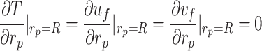10

During the simulation modeling process, a constant heat flux is applied to heat the low-temperature oil within the pipeline of specified dimensions, enabling the investigation of variations in thermophysical properties and heat transfer characteristics of the oil during heating transport; simultaneously, the influence of different oil mass flow rates on the heat transfer characteristics is examined. The geometric and boundary condition utilized are detailed in Table 1.

Table 1.

Boundary conditions in the simulation model.

Boundary condition	Fluid input conditions
	Mass flow rate G(kg/(m2·s))	Initial oil temperature t’f
value	180、360、540、720、900	20 ℃
Boundary condition	Boundary conditions for convective heat transfer
	Pipeline length Lp	Pipeline diameter Dp	Heat flux density q(W/m2)
value	10 m	0.06 m	1520、1920、2320、2720
Boundary condition	Fluid output conditions
	Gravitational g f	Outlet static pressure P0
value	9.81 m/s2	0 pa

Theoretical analysis of oil thermal coupling characteristics

Based on the dimensional analysis (Buckingham π theorem), the convective heat transfer coefficient and thermal boundary layer oil temperature during pipeline heating transport are nondimensionalized, yielding the coupling relationships of h and t_f with thermophysical properties (viscosity, density, specific heat capacity, thermal conductivity), flow parameters (velocity), and heat transfer surface characteristics (transport distance, pipeline diameter). The functional relationship of h with each parameter is expressed as:

11

Thus, the coupling functional relationship between the heat transfer coefficient and various parameters can be transformed into a dimensionless expression. Considering that the viscosity of oil exhibits a strong dependence on temperature, and the large temperature difference between the pipe wall and the fluid during the initial stage of transport leads to dynamic changes in viscosity during the transport process, a modified Nusselt number (Nu) correlation is introduced to address this issue:

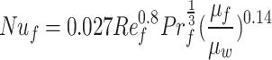12

where µ_f /µ_w is the temperature correction coefficient, and µ_f and µ_w are the dynamic viscosities of oil at its own temperature and the wall temperature, respectively (Pa·s). The hydrodynamic characteristics are characterized by the Reynolds number (Re) and Prandtl number (Pr), the definition formulas of the relevant parameters are as follows:

13

14

The above analysis indicates that the thermophysical parameters of oil (viscosity µ_f, density ρ_f, specific heat capacity (C_pf), thermal conductivity (λ)and flow parameters (velocity u_f and pipe diameter r) collectively determine the flow and heat transfer behaviors. Among them, viscosity and density dominate the flow state of oil, while viscosity, thermal conductivity, and specific heat capacity regulate the coupling relationship between the thermal boundary layer and flow boundary layer. To quantify the coupling effect of thermophysical parameters and the heat transfer process, a second expression for the Nusselt number is introduced, which is defined as the ratio of convective to conductive heat flux, with the expression:

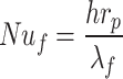15

Selecting ρ_f 、µ_f、λ_f 、r as fundamental physical quantities, dimensionless quantities are formed with h、u_f 、C_pf respectively, expressed in the power exponential form as follows:

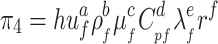16

In the above equation, the seven physical quantities are composed of the time dimension T, length dimension L, mass dimension M, and temperature dimension θ. The conversion of the above equation into the basic dimensional expression is as follows:

17

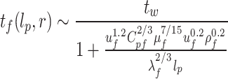
Using the principle of dimensional homogeneity, the solution yields a = b = 0.8, c=-7/15, d = 1/3, e = 2/3, f = 0.2. The equation for the influence of each parameter on the convective heat transfer coefficient between oil and the heating pipeline is as follows:

18

The energy transport equation for a specific oil section is expressed as follows:

19

In the process of processing the above equation, taking the temperature difference θ = t_f-t_w as the reference dimension (defined as the excess temperature), the dimensionless equation form is obtained as follows:

20

Integrating the above equation yields the relationship between the temperature change of the oil film near the wall and each parameter as follows:

21

Where θ₀ = t_f0-t_w is the initial temperature difference, which is jointly determined by the initial temperature of the oil and the heating temperature of the pipeline. Based on this, a coupling relationship model between the temperature of the oil in thermal boundary layer and key physical parameters is further established as follows:

22

Grid independence verification

Under operating conditions of heat flux density (q = 1520 W/m²) and mass flow rate (G = 900 kg/(m²·s)), numerical simulations are conducted to investigate the numerical solutions of four parameters under varying mesh densities during heating transport. Figure 4a presents the average boundary layer temperature of oil and the boundary layer outlet temperature of oil, while Fig. 4b shows Reynolds number (Re) and convective heat transfer coefficient (h). When the total number of grids reaches 1.69 × 10⁶, the impact of mesh refinement on the numerical solutions of these parameters diminishes, indicating numerical convergence at this mesh density.

Fig. 4.

Parameters under different grid numbers: (a) Average and outlet thermal boundary layer temperature; (b) Reynolds number and convective heat transfer coefficient.

As shown in Fig. 5, the numerical model is consisted of three components: the pipeline’s main body, oil region, and the intervening boundary layer between them. The pipeline has a diameter of 60 mm and a length of 10 m, with its geometry discretized via tetrahedral elements, Z resulting in 504,179 cells. The pipeline acts solely as a carrier for the constant heat flux density boundary condition and is coupled with the oil region, where meshing adheres to numerical stability criteria under thermal boundary layer. The oil region is discretized using tetrahedral meshes, yielding 963,010 cells. In contrast, the boundary layer between the pipeline and oil region, characterized by complex heat transfer processes and flow regimes, necessitates hexahedral prism elements for high-resolution mesh adaptation, ultimately yielding 222,016 cells to capture local flow and thermal gradient variations.

Fig. 5.

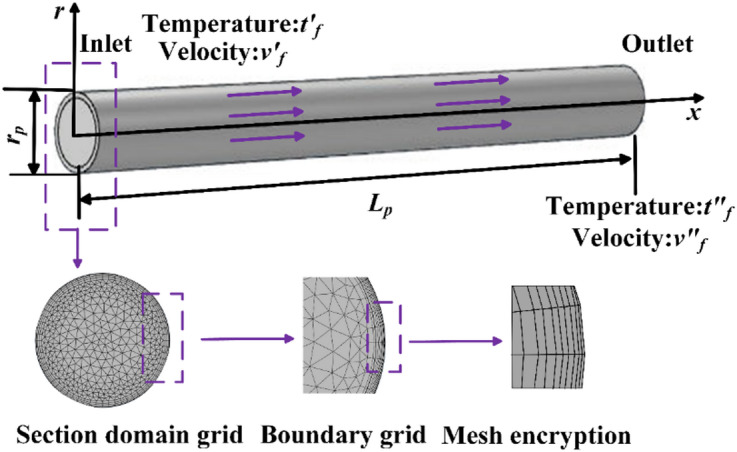
Numerical simulation meshing model. (r_p: Diameter of pipeline (m); L_p: Length of pipeline(m)).

Analysis and discussion of simulation results

Model verification

An experimental setup is established to validate the numerical model’s predictive accuracy, employing paraffin oil selected for its pronounced viscosity-temperature sensitivity as the experimental subject. Its viscosity-temperature relationship is experimentally measured (Fig. 6) and fitted to establish a benchmark for subsequent model validation.

Fig. 6.

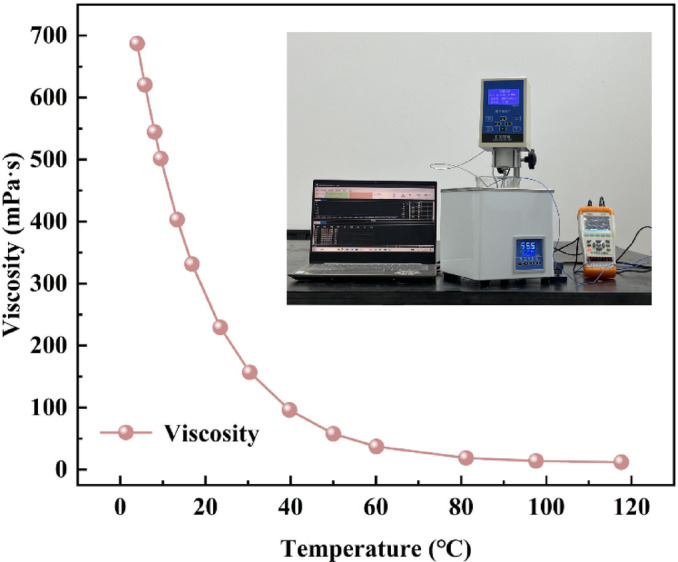
Viscosity-temperature characteristic curve of paraffin oil.

Significant temperature-dependent viscosity variation is demonstrated in Fig. 6.for oil entering the pipeline at 20 ℃. Model accuracy is validated through comparison of simulated oil outlet temperatures against theoretical calculations using the methodology established by Bimonte et al.³⁰. As shown in Fig. 7b, residual oil entering at 20 ℃ is heated by pipeline walls maintained at 80 ℃. Both approaches show consistent agreement along the transport distance, with maximum observed deviation between simulated and theoretical results remaining within acceptable engineering tolerance at 9.89%.

Fig. 7.

Model validation: (a) Experimental setup diagram; (b) Comparison of simulation and theoretical of oil outlet temperatures; (c) Comparison of simulation and experimental results of oil outlet temperature under different heating temperatures; (d) Comparison of simulation and experimental results of oil outlet temperature under different inlet temperatures.

The experimental setup for enhanced model validation (Fig. 7a) comprises an oil transport pipeline with an internal diameter of 22 mm and length of 1 m, externally wrapped with glass-fiber electric heating tape. An insulation layer of thermal conductivity 0.03 W/(m·℃) encases the assembly to minimize thermal dissipation. Thermal equilibrium was established through 30 min stabilization per test condition. Figure 7c and d show comparative experimental and simulation results for variations in pipeline heating temperature and oil inlet temperature, respectively. Experimental measurements reveal that the outlet temperature of the 18.9 ℃ initial temperature after transporting the heating pipeline aligns closely with numerical simulation results, achieving a maximum relative error of 5.14% and an average error of 4.04%, respectively. Systematic variation of heating temperature and oil inlet temperature validates model accuracy, demonstrating robustness against strong temperature-dependent viscosity effects. The reliability of thermophysical properties model is confirmed for predicting thermal coupling characteristics in deep-sea oil recovery processes under varying thermal conditions.

Thermal coupling characteristics of residual oil during heating transport

Under specified operating conditions (mass flux (G = 180 kg/(m²·s)), pipeline diameter (D = 0.06 m), and pipeline length (L = 10 m), the dynamic thermal coupling characteristics of low-temperature residual oil at 20 ℃ undergoing thermally driven transport in a high-temperature pipeline with a heat flux density of 1520 W/m² is analyzed. Thermal coupling characteristics across six axial segments are presented in Fig. 8.

Fig. 8.

Thermal coupling characteristics of oil during transport (a) The transport section; (b) The radial cross-section.

As shown in Fig. 8a, the experimental results indicate non-uniform temperature distributions within the same cross-section, where thermal boundary layer temperatures significantly surpass central-region values. Upon introduction of the oil with initial temperature at 20 ℃ into the heating pipeline, rapid temperature elevation (53.33 ℃ at 5 m) in thermal boundary layer is caused by thermal exchange with the high-temperature pipeline wall, and the temperature gradient of 6.43 ℃/m. Simultaneously, the central zone exhibits a minimal temperature rise of 1.4 ℃. This disparity arises from the laminar boundary layer effect in the wall zone (Fig. 8b), wherein the thermal boundary layer thickness expands from 10^− 5 mm to 5 × 10^− 4 mm by 5 m, accompanied by a temperature peak gradient of 39.44 ℃/mm within the boundary layer. Along the axial direction, the temperature gradient progressively diminishes to 0.41 ℃/m, and the oil temperature stabilizes at 59.24 ℃ by the 10 m mark. Furthermore, temperature differences between the front and rear wall zones exhibit a gradual decline along the axial direction: the initial disparity of 14.27 ℃ decreases to 5.64 ℃ at 5 m and diminishes to 0.74 ℃ by 10 m.

To elucidate the thermal coupling characteristics of oil, this study demonstrates the thermophysical properties of thermal boundary layer oil during transport, including temperature, density, specific heat capacity, and viscosity, and the heat transfer coefficient between the oil and the heating pipeline via numerical simulation, as shown in Fig. 9.

Fig. 9.

Thermal coupling characteristics of oil in thermal boundary layer during transport: (a) µ_f. (b) ρ_f. (c) C_pf. (d) h. (e) t_f. (f) Re.

The viscosity of thermal boundary layer oil sharply decreases from 277.99 mPa·s to 49.54 mPa·s during transport from 0 to 5 m as shown in Fig. 9a, while density and specific heat capacity exhibit linear axial reductions characterized by coefficients of K_ρf =-7.19 kg/m⁴ and K_Cpf =-241.08 J/(kg·℃·m) respectively as shown in Fig. 9b and c.Viscosity variation is identified as the primary driver of flow regime transitions. Beyond the 5 m transport point, the axial variations of oil thermophysical properties stabilize with sharply decreasing rates. The temperature sensitivity of viscosity (dµ/dT) decreases from − 6.85 mPa·s/℃ to − 1.91 mPa·s/℃, indicating weakened intermolecular forces at elevated temperatures and diminished viscosity sensitivity to temperature fluctuations, thereby reducing flow resistance. Simultaneously, specific heat capacity shows an anomalous slight increase from 2007.5 to 2011.1 J/(kg·℃), attributed to enhanced molecular vibrational degrees of freedom, which elevate heat storage capacity per unit mass. These property changes affect thermal coupling characteristics, stabilizing the convective heat transfer coefficient at 50.85 W/(m²·℃) by the 8 m mark. Concurrently, temperature increase rates gradually diminish and converge to 58.94 ℃.

According to the Eq. 23, under fixed pipeline dimensions and thermal conductivity, the sustained temperature fields rise is governed by negative correlations between thermophysical properties, accumulated thermal energy, and enhanced flow dynamics. During the initial heating phase, thermophysical properties exhibit pronounced temperature sensitivity, with variations observed in the thermal boundary layer oil as temperature rises. When the oil is transported from 2 m to 5 m, the convective heat transfer coefficient increases from 20.23 to 40.58 W/(m²·℃) in Fig. 9d, accompanied by a temperature increase from 32.53 ℃ to 53.33 ℃. Beyond 8 m, viscosity, specific heat capacity, and density demonstrate diminished temperature dependence and stabilize at 0.22 mPa·s, 2023.3 J/(kg·℃), and 859.98 kg/m³ respectively. Concurrently, the convective heat transfer coefficient stabilizes at 50.85 W/(m²·℃) while the boundary layer oil temperature remains constant at 58.64 ℃.

As established by Eq. 18 under specified pipeline dimensions, the convective heat transfer coefficient at the thermal boundary layer and pipe wall interface is determined to scale with thermophysical properties through the following exponential dependencies. Despite the concurrent reductions in specific heat capacity and viscosity being observed to suppress heat transfer augmentation, the dominant rapid viscosity reduction is demonstrated to strengthen flow dynamics, consequently intensifying convective heat transfer. In Fig. 9e, the temperature of thermal boundary layer oil rises rapidly, exceeding the wax appearance temperature of 46.42 ℃ at 5 m and thereby initiating dissolution of entrained solid wax. Upon saturation of latent heat absorption during solid wax phase transport, conductive heat transfer dominates, leading to a decline in specific heat capacity. Collective molecular motions increase intermolecular spacing, thereby reducing density. Concurrently, elevated temperatures weaken wax crystal skeletal structures, expanding free volume and diminishing intermolecular forces, thereby lowering viscosity. the Re increases to 312.58 at 5 m, transitioning the oil flow from a pseudo-plastic non-Newtonian state to a laminar regime as shown in Fig. 9f. The velocity field exhibits a parabolic distribution, reaching a maximum central velocity of 1.98 m/s. Increased boundary layer turbulence enhances heat transfer mechanisms between the thermal boundary layer oil and the heating transport pipeline, elevating the convective heat transfer coefficient to 40.58 W/(m²·℃).

Changing law of thermal physical properties of residual oil under different heat flux density

Illustrated in Fig. 10a, the thermal boundary layer oil temperature under a mass flux of 180 kg/(m²·s) is examined under constant heat flux conditions. With heat flux increased in 400 W/m² increments, the boundary layer temperature gradient response is intensified, while the temperature difference between thermal boundary layer oil and central fluid at the pipeline outlet exhibits near-linear growth. Concurrently, the internal oil temperature field demonstrates minimal thermal elevation as depicted in Fig. 10b. These observations indicate that elevated heat flux gradients are observed to enhance convective heat transfer efficiency near the wall while simultaneously amplifying radial temperature gradient non-uniformity.

Fig. 10.

Schematic illustration of temperature field variations in oil under different heat flux densities at a constant mass flux of 180 kg/(m²·s): (a) Thermal boundary layer oil temperature. (b) Radial sectional temperature field of oil at intervals of 2 m during transport.

In order to further investigate heat flux density effects on thermal coupling characteristics, as shown in Fig. 11, the properties including temperature, viscosity, density, specific heat capacity, and convective heat transfer coefficient at the thermal boundary layer after flowing through a 10 m heating pipeline is investigated as a function of heat flux density.

Fig. 11.

Effect of heat flux density s on oil transport characteristics under a prescribed mass flux.

It is shown that oil temperature and temperature gradient (∆t_f/∆x) increase with heat flux density during initial transport phases. However, temperature gradient responses demonstrate delayed progression under elevated mass flux conditions. Figure 11a demonstrates that under G = 180 kg/(m²·s), temperature peak gradient consistently occurs at 1 m as heat flux density increases in 400 W/m² increments. The temperature peak region, defined as a localized domain where the oil temperature exceeds both the inlet and bulk average temperatures due to incomplete thermal mixing, viscous dissipation, and asymmetric heating effects, is observed to undergo a downstream displacement to the 3 m position when the mass flux is elevated to 900 kg/(m²·s) in Fig. 11e. Concurrently, the temperature peak gradient exhibits a monotonic increase with rising heat flux density, attaining progressively higher values of 10.08, 12.84, 15.53, and 18.22 ℃/m. At the outlet, gradients further decline to below 0.5 ℃/m, achieving thermophysical equilibrium.

At low mass fluxes ranging from 180 to 540 kg/(m²·s), the outlet temperature exhibits a linear relationship with heat flux density, governed by a proportionality coefficient K = 0.04. This relationship maintains a constant temperature difference of ΔT ≈ 0.04 ℃/(W/m²) between thermal boundary layer and heating pipeline heat flux gradients. When the mass flux increases to 720 kg/(m²·s), the proportionality coefficient decreases to K = 0.03, resulting in a 30% reduction in temperature regulation efficiency. This reduction is attributed to dual constraints: shortened residence time and thickening thermal boundary layers at high flow rates. All operational conditions yielded outlet temperatures above 60℃, enabling near-complete dissolution of oil and optimal transport conditions. Thermophysical properties analysis shows that density decreases monotonically with increasing heat flux density. The specific heat capacity shows a turning point above 50℃, transitioning from a decreasing to an increasing trend that correlates positively with temperature (0.19% increase). The temperature sensitivity of viscosity diminishes at elevated temperatures as intermolecular forces weaken. Convective heat transfer analysis reveals a positive correlation between the convective heat transfer coefficient and density/specific heat capacity, and an inverse relationship with viscosity. Under these parameter influences, the ratio of convective heat transfer coefficient to heat flux density increases from K = 0.018 to K = 0.041 when the mass flux is 180 kg/(m²·s).

Changing law of thermal physical properties of residual oil under different mass flux

The influence of mass flux (180, 360, 540, 720, and 900 kg/(m²·s)) on thermal coupling characteristics across heat flux densities from 1520 to 2720 W/m² is presented in Fig. 12. Specifically, under a constant heat flux density of 1520 W/m², the outlet temperature of oil in thermal boundary layer decreases by 10.73 ℃ when mass flux increases from 180 to 900 kg/(m²·s). The convective heat transfer coefficient exhibits a parallel decline, with both parameters showing higher response magnitudes than low heat flux density conditions. Among thermophysical properties, viscosity is most sensitive to mass flux variations, highlighting a dominant heat transfer-flow coupling mechanism between mass flux and heat flux density. When the heat flux density increases from 1520 W/m² to 2720 W/m², the temperature rise reaches 52.19 ℃ at a mass flux of 180 kg/(m²·s), while it decreases to 39.43 ℃ at 900 kg/(m²·s), representing a 24.5% reduction compared to the lower mass flux condition. This discrepancy arises from two competing mechanisms: enhanced heating transport due to reduced boundary layer thickness caused by increased velocity ((u = G/(ρA)), and weakened heat absorption resulting from shortened residence time (t = L/u). The latter mechanism dominates, resulting in reduced overall heat transfer efficiency, as indicated by the observed temperature decline in the oil boundary layer under higher mass flux conditions. Based on the observed thermophysical properties, a segmented control strategy is formulated to optimize the heating transport. At low heat flux density conditions, a moderate mass flux of 360–540 kg/(m²·s) is employed to prolong residence time and enhance heat retention. At high heat flux density condition a mass flux of ≥ 900 kg/(m²·s) is applied to intensify convective heat transfer, while residence time regulation minimizes localized overheating risks and prevents thermal cracking. This strategy achieves a balance between heat transfer efficiency and thermal safety, optimizing both parameters simultaneously.

Fig. 12.

Effect of mass flux on oil transport characteristics under a prescribed heat density.

Conclusion

A numerical model was developed for the deep-sea low-temperature oil thermos-fluid coupled system based on thermophysical properties of oil. Multi-field coupling theoretical analysis was conducted on the temperature of oil in thermal boundary layer and the convective heat transfer coefficient, systematically elucidating the regulatory mechanisms of thermal coupling characteristics by transport distance, heat flux density, and mass flux. The study further reveals that:

1. The convective heat transfer coefficient between the thermal boundary layer oil and the pipe wall exhibits positive correlations with density, specific heat capacity, and thermal conductivity, while inversely correlating with dynamic viscosity. Although reduced density and specific heat capacity of residual oil suppress its enhancement during heating transport, the rapid decline in viscosity (76.76% reduction at x = 5 m) intensifies convective heat transfer by improving boundary layer fluidity. This viscosity-driven flow enhancement elevates the Reynolds number to 312.58, establishing both the axial temperature peak gradient of 6.43 ℃/m and heat transfer coefficient increasing to 40.58 W/(m²·℃). Beyond 7 m, the axial temperature gradient diminishes to 0.62 ℃/m as the boundary layer stabilizes at 58.94 ℃. These results confirm that viscosity variation governs both flow state transition and thermal boundary layer restructuring, thereby regulating temperature gradient evolution.

2. Heat flux density governs the residual oil temperature field in the pipe wall region, where its elevation enhances the thermal driving force and intensifies boundary layer temperature gradients. Under low mass flow conditions, oil temperature at x = 10 m exhibits a linear response to heat flux density (slope K = 0.04 ℃·m²/W).When mass flux increases to 900 kg/(m²·s), stepwise heat flux increments from 1,520 to 2,720 W/m² (Δq = 400 W/m²) elevate the temperature peak region from 1 m to 3 m section, with measured values of 10.08, 12.84, 15.53, and 18.22 ℃/m. Thermal regulation efficiency of heat flux diminishes under these elevated mass flux conditions relative to low mass flux operation, evidenced by a reduction in the heat transfer coefficient from 124.74 to 46.36 W/(m²·℃).

3. The heat transfer process exhibits dual dependence of mass flux: Under low mass flow (0.5 kg/s), the temperature rise rate peak at 19.67 ℃/m within the initial 1-m section. At elevated mass flow (2.5 kg/s), increased velocity enhances convective heat transfer while reduced residence time attenuates thermal accumulation, resulting in spatially delayed temperature gradients. This regime shifts the peak temperature rise rate to 10.08 ℃/m and relocates its temperature peak region occurrence to the 1–3 m section. Despite improved convective efficiency at higher mass flux, limited thermal exposure prevents substantial bulk temperature elevation.

Abbreviations

A_p

Pipeline cross-section area [m²]

C_f

Specific heat capacity of the oil [J/(kg·℃)]

C_pf

Specific heat capacity of a pipeline [J/(kg·℃)]

D_p

Pipeline diameter [mm]

f

Coefficient of resistance to flow in the pipeline

g_f

Oil gravity [m/s²]

h_f

Oil convection heat transfer coefficient [W/(m²·℃)]

l_p

Pipeline length [m]

Nu_f

Dimensionless temperature gradient of oil in the adherent layer

Pr_f

Ratio of oil momentum diffusion capacity to heat diffusion capacity

M_f

Oil mass velocity [kg/(m²·s)]

Q_p

Heat flow density for convective heat transfer from pipeline to oil [W/m²]

r_p

Pipe diameter [m]

Re_f

Ratio of inertial force to viscous force of oil itself

t’_f

Oil initial temperature [℃]

t"_f

Oil outlet temperature [℃]

tw

Heating pipeline temperature

u_f

Oil velocity [m/s]

u’_f

Inlet velocity [m/s]

u"_f

Outlet velocity [m/s]

λ_p

Pipeline thermal conductivity [W/(m·℃)]

λ_f

Oil thermal conductivity [W/(m·℃)]

µ_f

Oil viscosity [mPa·s]

µ_w

Dynamic viscosity of oil at pipeline temperature [mPa·s]

Ʈ

Frictional stress per unit area of oil flowing in a pipeline [Pa]

ρ_f

Oil density [kg/m³]

ρ_p

Pipeline density [kg/m³]

Author contributions

B. prepared the overall framework of the paper and Figure 1; L. conducted the theoretical analysis of the paper and constructed a coupling model; M. prepared various materials during the process; S. prepared the data processing during the experimental process; W. prepared the theoretical analysis part of the simulation process, and G. conducted Figs. 9 and 10.

Funding

Financial support from the National Key Research and Development Program of China (Grant No. 2023YFC2809704), the National Natural Science Foundation of China General Project (Grant No. 52571280). And the Doctoral Start-up Foundation of Liaoning Province (Grant No. 2025-BS-0223).

Data availability

The datasets used and/or analyzed during the current study available from the corresponding author on reason able request.

Declarations

Competing interests

The authors declare no competing interests.

References

- 1.Sun, Q. et al. Insights into enhanced oil recovery by thermochemical fluid flooding for ultra-heavy reservoirs: an experimental study. Fuel331, 125651. 10.1016/j.fuel.2022.125651 (2023). [Google Scholar]
- 2.Feng, X. & Zhang, B. Applications of bubble curtains in marine oil spill containment: hydrodynamic characteristics, applications, and future perspectives. Mar. Pollut Bull.194, 115371. 10.1016/j.marpolbul.2023.115371 (2023). [DOI] [PubMed] [Google Scholar]
- 3.Cao, W. et al. A novel integrated method for heterogeneity analysis of marine accidents involving different ship types. Ocean. Eng.312, 119295. 10.1016/j.oceaneng.2024.119295 (2024). [Google Scholar]
- 4.Nian, T., Guo, X., Fan, N., Jiao, H. & Li, D. Impact forces of submarine landslides on suspended pipelines considering the low-temperature environment. Appl. Ocean. Res.81, 116–125. 10.1016/j.apor.2018.09.016 (2018). [Google Scholar]
- 5.Zhao, J., Dong, H., Wang, X. & Fu, X. Research on heat transfer characteristic of crude oil during the tubular heating process in the floating roof tank. Case Stud. Therm. Eng.10, 142–153. 10.1016/j.csite.2017.05.006 (2017). [Google Scholar]
- 6.Huerta, F. & Vesovic, V. CFD modelling of the non-isobaric evaporation of cryogenic liquids in storage tanks. Appl. Energy. 356, 122420. 10.1016/j.apenergy.2023.122420 (2024). [Google Scholar]
- 7.Zhao, J., Dong, H., Wei, L. & Zhou, G. Research on heat transfer characteristic of waxy crude oil after oil pipeline shutdown. J. Therm. Anal. Calorim.129, 487–508. 10.1007/s10973-017-6121-y (2017). [Google Scholar]
- 8.Xie, H., Li, C., Wei, N., Zhang, C. & He, J. Numerical study on the optimal thermally affected region of a buried oil pipeline. ACS Omega. 8, 27761–27775. 10.1021/acsomega.3c03945 (2023). [DOI] [PMC free article] [PubMed] [Google Scholar]
- 9.Li, Y., Su, H., Jiang, W., Cai, Z. & Chen, J. Sealing performance of subsea Wellhead connector under thermal-structural coupling. Ocean. Eng.270, 113504. 10.1016/j.oceaneng.2022.113504 (2023). [Google Scholar]
- 10.Zhang, L., Du, C., Wang, H. & Zhao, J. Three-dimensional numerical simulation of heat transfer and flow of waxy crude oil in inclined pipe. Case Stud. Therm. Eng.37, 102237. 10.1016/j.csite.2022.102237 (2022). [Google Scholar]
- 11.Zeng, Z. et al. Effect of the dynamic humid environment in salt caverns on their performance of compressed air energy storage: A modeling study of thermo-moisture-fluid dynamics. Appl. Energy. 377, 124403. 10.1016/j.apenergy.2024.124403 (2025). [Google Scholar]
- 12.Dolatyari, A., Ahmady, M. & Kazemi, A. A novel mathematical model for modeling viscosity and temperature relationship for dead oils. Sci. Rep.14, 22836. 10.1038/s41598-024-73573-8 (2024). [DOI] [PMC free article] [PubMed] [Google Scholar]
- 13.Nian, T., Gu, Z., Guo, X., Zhang, H. & Jia, Y. Effect of temperature rise on the mechanical behaviour of deep-sea clay surrounding oil and gas pipelines. Ocean. Eng.302, 117533. 10.1016/j.oceaneng.2024.117533 (2024). [Google Scholar]
- 14.Fu, C. et al. Analysis of subsidence patterns of the formation around the wellbore during deepwater natural gas hydrate test production conditions. Appl. Ocean. Res.153, 104257. 10.1016/j.apor.2024.104257 (2024). [Google Scholar]
- 15.Zhao, W., Zhao, J., Si, M. & Liu, J. Thermal characteristics of waxy crude oil during its static cooling in an overhead pipeline. Case Stud. Therm. Eng.14, 100475. 10.1016/j.csite.2019.100475 (2019). [Google Scholar]
- 16.Yang, M. et al. A novel method for estimating transient thermal behavior of the wellbore with the drilling string maintaining an eccentric position in deep well operation. Appl. Therm. Eng.163, 114346. 10.1016/j.applthermaleng.2019.114346 (2019). [Google Scholar]
- 17.Ali, Q., Younas, U., Farman, M. & Amir, M. Prabhakar fractional simulation for thermal analysis of magnetohydrodynamics flow of Oldroyd-B fluid using slip and newtonian heating effects. J. Therm. Anal. Calorim.10.1007/s10973-024-13514-9 (2024). [Google Scholar]
- 18.Ma, X., Sun, Y., Guo, W., Jia, R. & Li, B. Numerical simulation of horizontal well hydraulic fracturing technology for gas production from hydrate reservoir. Appl. Ocean. Res.112, 102674. 10.1016/j.apor.2021.102674 (2021). [Google Scholar]
- 19.Abdelhafiz, M. M., Hegele, L. A. Jr & Oppelt, J. F. Numerical transient and steady state analytical modeling of the wellbore temperature during drilling fluid circulation. J. Pet. Sci. Eng.186, 106775. 10.1016/j.petrol.2019.106775 (2020). [Google Scholar]
- 20.Sanchez, S. et al. Conjugate thermal-hydrodynamic model for the study of heavy oil transport. J. Pet. Sci. Eng.179, 997–1011. 10.1016/j.petrol.2019.04.083 (2019). [Google Scholar]
- 21.Xu, Y. et al. Heat transfer characteristics of cascade phase change energy storage composite pipeline. Heat. Mass. Transf.60, 1441–1452. 10.1007/s00231-024-03497-6 (2024). [Google Scholar]
- 22.Xie, H., Li, C., Jia, W., Zhang, C. & Three-Dimensional, C. F. D. Modeling on the thermal characteristics of buried oil pipeline involving the heat transfer of wax layer. Energies15, 6022. 10.3390/en15166022 (2022). [Google Scholar]
- 23.Dong, H., Zhao, J., Zhao, W., Si, M. & Liu, J. Study on the thermal characteristics of crude oil pipeline during its consecutive process from shutdown to restart. Case Stud. Therm. Eng.14, 100434. 10.1016/j.csite.2019.100434 (2019). [Google Scholar]
- 24.Wang, Y., Quan, Q., Dai, K., Wang, S. & Yuan, Z. Quantitative effects of different factors on the thermal characteristics of new submarine hot oil pipeline during the preheating process. Chem. Tech. Fuels Oils. 58, 653–664. 10.1007/s10553-022-01433-0 (2022). [Google Scholar]
- 25.Li, W., Chen, L., Zhao, J. & Wang, W. Mechanism and Data-Driven dual Estimation of coupling Hydraulic-Thermal States for steam heating networks considering Multi-Time-Scale characteristics. IEEE T Cybern. 54, 4567–4580. 10.1109/TCYB.2023.3312699 (2024). [DOI] [PubMed] [Google Scholar]
- 26.Duan, J. et al. Predicting temperature distribution in the waxy oil-gas pipe flow. J. Pet. Sci. Eng.101, 28–34. 10.1016/j.petrol.2012.10.003 (2013). [Google Scholar]
- 27.Salahuddin, T. & Awais, M. Cattaneo-Christov flow analysis of unsteady couple stress fluid with variable fluid properties: by using adam’s method. Alexandria Eng. J.81, 64–86. 10.1016/j.aej.2023.09.021 (2023). [Google Scholar]
- 28.Ramos-Pallares, F., Schoeggl, F. F., Taylor, S. D. & Yarranton, H. W. Prediction of thermal conductivity for characterized oils and their fractions using an expanded fluid based model. Fuel234, 66–80. 10.1016/j.fuel.2018.06.112 (2018). [Google Scholar]
- 29.Sun, W. et al. Heat flow coupling characteristics analysis and heating effect evaluation study of crude oil in the storage tank different structure coil heating processes. Int. J. Heat Mass Transf.127, 89–101. 10.1016/j.ijheatmasstransfer.2018.08.035 (2018). [Google Scholar]
- 30.Bimonte, G., Emig, T., Kardar, M. & Krüger, M. Nonequilibrium fluctuational quantum electrodynamics: heat Radiation, heat Transfer, and force. Annu. Rev. Condens. Matter Phys.8, 119–143. 10.1146/annurev-conmatphys-031016-025203 (2017). [Google Scholar]
Associated Data
This section collects any data citations, data availability statements, or supplementary materials included in this article.
Data Availability Statement