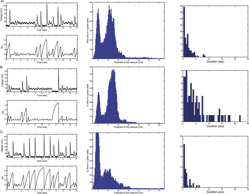
Figure 2. Up–Down State Dynamics under Normal and Clamp Conditions.
(A) A typical realization of Up–Down transition dynamics in the stochastic model with wT = 12.6.
Top graph: (Up) average population voltage (mV), baseline at 0 mV; (Down) plot of the depression variable μ as a function of time: when the system arrives in the Down state, it is depressed. Then the depression recovers slowly toward 1. Usually the noise is able to produce a transition, before full recovery is achieved.
Bottom graph: Histogram of the population voltage: fraction of the time spent in a given state. Units are in ms on the y-axis and in mV on the x-axis: the fraction of total time spent in the Up and Down state is about the same during the 20 s of simulations. The maximum time in the Up state is about 500 ms but the mean maximum time is about 3 s.
Right column graph of (A): histogram of the duration of the Up states.
(B) Effect of an external stimulation: depolarization. When a constant external input (I = 0.8) is added into the model, the neural network spends on average more time in the Up state than in Down state. In that case, the attractor point P 1 is shifted and is now closer to the separatrix.
(C) Hyperpolarization, simulated by a current injection. A hyperpolarization (I = −0.3) drives the ensemble of neurons at a lower mean potential, and as a result the neural network spends on average more time in the Down state.

