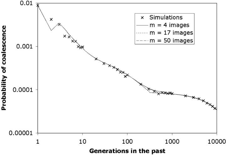
Figure 8.—

Effect of image number on the coalescence time probability distribution. The distribution of coalescence times was determined using three different choices for the number of images (m = 4, 17, and 50). The habitat is a 10 × 10 square with ρ = 100 and σ = 0.3 (N = 10,000; Nb = 113). The samples are from adjacent locations at (1.95, 2.0) and (2.05, 2.0). The effective population size from Equation 6 is 10,669. The transition times were determined from Equation 7: τ = 308 for m = 4; τ = 454 for m = 17; τ = 759 for m = 50. Crosses indicate the probability distribution determined from 100,000 simulated coalescence times. Older coalescence rates represent the average rate over a range centered on that marker. For example, the mark at t = 30 represents the average rate from t = 25–35; the mark at t = 3000 is the average from t = 2500–3500. The predicted coalescence probability distribution is very similar for the different values of m except in the vicinity of the transition between the scattering and collecting phases. The dip in the analytic values at t = 2 results from the fact that this probability distribution was derived by subtracting the CDF at t − 1 from the CDF at t. The CDF determined by Equation 2 significantly underestimates the probability of coalescence for very small values of T, and the value of the CDF at T = 1 was taken simply to be 1/Nb.