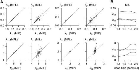
FIGURE 6.
Comparison between discrete-time and continuous-time maximum-likelihood algorithms. One-hundred data sets, each 100-s long, sampled at 10 Hz, were simulated with the nonperiodic model closed-open-closed (k12 = 0.1 s−1, k21 = 0.05 s−1, k23 = 5.0 s−1, and k32 = 2.0 s−1), and were maximum likelihood-fit individually. We tested the following algorithms: MIP (discrete-time, presented in this article), MPL (discrete-time) (17), and MIL (continuous-time, first-order missed events correction) (19). (A) Cross-correlation plots show that estimates obtained with MIP (x axis) match almost perfectly the estimates obtained from the same data set with MPL (y axis), and are well correlated with the estimates obtained with MIL (y axis). Notice that MIL's estimates have greater variance than those obtained with the other two algorithms. (B) Estimates obtained with MIL may depend critically on the choice of dead-time parameter for missed event correction. In the example shown, the best values were obtained with a dead-time ≈1.6 × dt, where dt is the sampling interval. MIP and MPL do not require missed event correction. The dotted lines mark the true parameter values.

