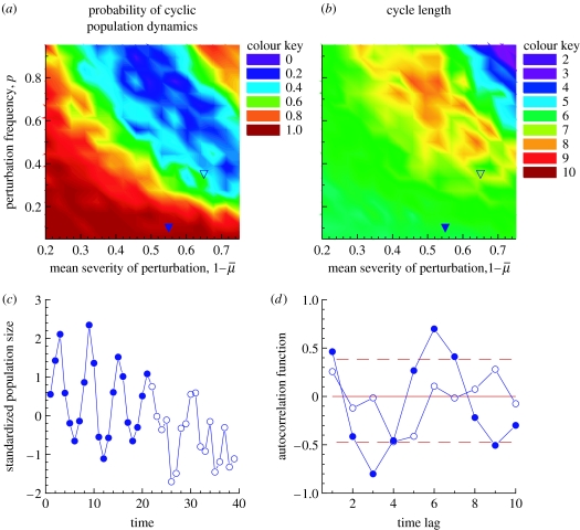
Figure 4.

Contour plots for the probability of (a) cyclic population fluctuations and (b) cycle length as a function of the mean severity of perturbation, 1−$\overline{\mu }$ and frequency, p, of an environmental perturbation. In (a) and (b) we have marked two points in the parameter space where the Finnish grouse dynamics could have been originally (filled triangle) and where they could be now (empty triangle). (c) shows a typical example of the resulting population fluctuations if the original parameters shift in time ($\overline{\mu }$ (t)=0.45−0.0025t; p(t)=0.1+0.009t). The first and second part of the time-series is depicted with different colours to demonstrate how the population dynamics change. The autocorrelation functions for these two parts of the time-series are shown in (d) with corresponding symbols.