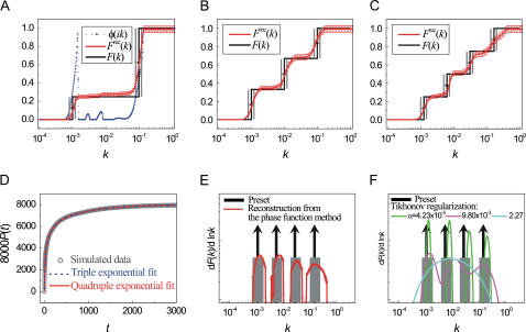
FIGURE 4.

Reconstruction of discrete F(k) from simulated kinetic data p(t). (a–c) Comparison between the F^rec(k) reconstructed from p(t) using the phase function approach (red line) and the preset F(k) (black line). Gray bars indicate the natural finite sampling width set by the Poisson noise arising from sampling only a finite number (8000) of dwell times. (d) Triple (blue dotted line) and quadruple (red solid line) exponential fittings of the time domain data (gray symbols), simulated using the preset F(k) depicted in panel c. (e) Comparison between the probability density dF(k)/d ln k reconstructed using the phase function approach (red line) and the preset probability density (black arrows and gray columns). The probability density functions (dF(k)/d ln k) were derived from rate constant distributions (F(k)) shown in panel c. The black arrows indicate the locations of the discretely distributed rate constants and the gray columns describe the natural finite sampling width. (f) The rate constant probability density reconstructed from the time domain data using the inverse Laplace transform with Tikhonov regularization. The time domain data was generated from F(k) shown in panel c. Different colored lines correspond to different values of the Tikhonov penalization parameter α. The preset probability density (black arrows and gray columns) is shown for comparison.