Evaluation of mortality trajectories in evolutionary biodemography

Abstract

An important task in evolutionary biodemography is to determine the schedule of survival and reproduction as the outcome of natural selection acting on life histories. We do this by using a model in which the state of the organism is characterized by mass and accumulated damage, both of which are affected by activity and which affect the rate of mortality. Focusing on growth during the juvenile period, we determine the level of activity that maximizes reproductive value. Given this, we are able to project forward and determine the trajectory of mortality for an individual following the optimal life history, given the physiological and reproductive parameters. We show that there are two main classes of juvenile mortality trajectories: U-shaped (such as recently reported for prereproductive humans) and steadily declining and we are able to connect the shape of the mortality trajectory with the physiological and reproductive parameters characterizing the life history. Our work shows the importance of state in models of evolutionary biodemography and the power of modern computational methods to illuminate biological process.

Demography is, in part, the study of the implications of a schedule of survival and mortality. The goal is to describe patterns, understand pattern and process, and predict the consequences of change on those patterns. Evolutionary biodemography asks about the origins of such schedules, in the context of evolution of life histories by natural selection. Evolutionary biodemography seeks to merge demography with evolutionary thinking (2–6). The result, for example, will be to use the comparative method to explore similarities and differences of patterns across species and to understand the patterns and mechanisms of vital statistics as the result of evolution by natural (and sometimes artificial) selection. Raymond Pearl, one of the founders of quantitative population biology, understood the importance of doing this but lacked the mathematical tools to do so. For example, with John Miner (7) he wrote “For it appears clear that there is no one universal ‘law’ of mortality…different species may differ in the age distribution of their dying just as characteristically as they differ in their morphology” and that “But what is wanted is a measure of the individual's total activities of all sorts, over its whole life; and also a numerical expression that will serve as a measure of net integrated effectiveness of all of the environmental forces that have acted upon the individual throughout its life”. With the development of state-dependent life history theory (8–10), the tools now exist.

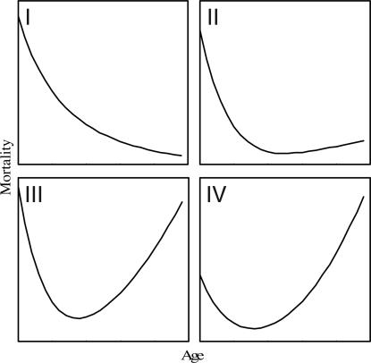
Here we respond to the challenge of Wachter (11), who noted that the evolutionary theories of aging generally fail to be able to predict the characteristics of mortality trajectories. To do this, we apply a recent development in state-dependent life history theory (12) that accounts for activity, the generation of cellular damage through metabolism and reinforcement of damage, repair of damage, and the mortality consequences of damage. This approach may be thought of as a fusion of the free-radical theory of aging (13) and the disposable soma theory (14) in an optimal life history context. Other efforts along these lines have developed simplified models with limited numbers of parameters (15, 16) or constructed models specific to a given system (17–19). In framing the aging problem as one driven by energy acquisition as well as allocation, our model is analogous to that recently developed by Yearsley et al. (20). However, our approach differs from these prior approaches in three important respects. First, the mortality trajectories we find are not a priori governed by a particular functional form but rather are an emergent property of the life history optimization. Thus, the range of trajectories that are possible is not constrained to lie within some traditional family of functions. Second, we focus on the development of mortality trajectories before the onset of maturation. Clearly, this departure from the traditional approach leaves open the question of what happens after maturation. Nevertheless, we obtain worthwhile insights into the shape of prereproductive mortality trajectories. Third, rather than focusing on parameters attributable to a particular species, we attempt to enumerate all of the trajectory shapes possible within a fairly broad range of the parameter space. We used 3,000 parameter sets to characterize the mortality trajectories that this framework is capable of producing. After visual inspection of all 3,000 optimal mortality trajectories, four main classes of shapes emerged (Fig. 1). We tabulated the frequency with which each trajectory shape occurred and note the fitness and final size associated with each trajectory. We categorized the kinds of mortality trajectories that result from the life history and interpret our results in that context. (More details are given in Materials and Methods).

Fig. 1.

The four classes of mortality trajectories produced by our modeling framework are steadily declining or broadly U-shaped.

Results

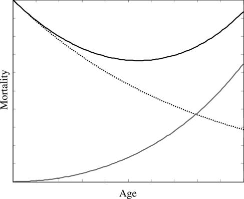
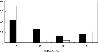
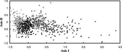
As in ref. 12, rather than fit the model to a particular data set, we sampled the parameter space (Table 1) and examined the resulting mortality trajectories. In addition to finding that a variety of trajectories are possible (also see ref. 21), ranging from Gompertz like behavior to declines of mortality rate, we are able to decompose the mortality trajectory into size dependent and damage dependent components (Fig. 2). Because we compute the fitness associated with a set of parameter values, we are also able to compute both raw and fitness-normalized frequencies of each class of mortality trajectory (Fig. 3). Finally, although the relationship between the physiological parameters and the mortality trajectory they produce is quite complicated, a discriminant function based on the parameters and all possible first order interactions explains 90% of the variability in parameter space among trajectory types and provides a simple means to visualize these relationships (Fig. 4).

Table 1.

Summary of the parameter space searched

Parameter	Description	Range searched
ζ	Maximum consumption rate	4–4.5
κ	Half-saturation consumption	0.1–0.2
μa	Activity-dependent mortality	1–10
ρD	Damage reinforcement rate	0–0.01
ρR	Energy-to-damage conversion	0.001–1
μD	Damage-dependent mortality	0.0001–0.5
ν	Energetic efficiency of repair	0.1–1
η	Maximum repair rate	0–1
β	Half saturation for repair	0–8
φX	Value exponent for size	0.001–10
φD	Value exponent for damage	0.001–10

Fig. 2.

Decomposition of the mortality trajectory into size- and damage-dependent components. The solid line indicates the total mortality as represented in Fig. 1. The dotted line indicates the size-dependent mortality, whereas the dashed line indicates damage-dependent mortality.

Fig. 3.

Frequencies of each mortality trajectory. Filled bars indicate the raw frequencies of each trajectory type, open bars indicate the geometric mean fitness-weighted frequencies of each.

Fig. 4.

Linear discriminant function analysis of the parameters and first-order parameter interactions associated with each type of mortality trajectory. Trajectory types are indicated by the different marker types and line up along the horizontal axis in order. That is, trajectory types I–IV are indicated by the gray circles, black circles, white squares, and gray squares, respectively.

Discussion and Conclusion

Our approach to the computation of mortality trajectories in evolutionary biodemography is based on phenotypic modeling; in this sense it is a version of the disposable soma theory (22,23). However, we are able to reproduce the U-shaped trajectories that are commonly observed in natural, human and engineering systems. In our model, in all cases the early decline of mortality is due to the decline of size dependent mortality, which decreases as the organism grows and the increased mortality later in life is due to the accumulation of damage. Thus, our phenotypic theory developed for prereproductive individuals, can predict the common U-shape of mortality trajectories, something that purely genetic theories are currently unable to do (and noted by Hamilton in his original work; ref. 24). Although type I and II curves are considered more typical for prereproductive intervals, recent analyses for humans (25) revealed a U-shaped trajectory before maturation providing striking empirical support for the type III and IV curves.

There is no simple relationship between the values of the physiological parameters and the mortality trajectories they generate. For any given parameter, we find trajectories from each class throughout the sampled range. However, within this highly complicated space, there is a single discriminant axis along which there is a smooth transition from declining to increasing mortality (Fig. 4), which is dominated by interactions among parameters. The loadings on this axis (Table 2) allow us to interpret the conditions under which each mortality trajectory may occur. For example, trajectories in class 1, for which mortality continues to decline are characterized by high rates of consumption and activity, relatively high damage accumulation, and very low dependence of mortality and reproductive value upon damage. This class of trajectory represents ≈50% of the simulated parameter values and is commensurately common among juveniles in natural or human systems. On the other hand, trajectories in which mortality is increasing with age are characterized by high sensitivity of fitness to damage. Although we focus on a juvenile period, these results suggest that increasing late-life mortality trajectories are common in nature because accumulated damage incurs nonnegligible fitness costs. We also note that the rise in mortality rates with increasing age cannot be simply due to the use of a fixed end of the juvenile period because the rise in mortality rates does not occur in the majority of parameter sets. Furthermore, other models (16–18) using the same general approach (but for very different specific problems) that allow for reproduction before the final time period also show the rise in mortality.

Table 2.

Loadings for the 30 most important parameter combinations determining the shape of the mortality trajectories

Parameter combination	Loading on axis 1	Loading on axis 2	Parameter combination	Loading on axis 1	Loading on axis 2
ζ × κ	−0.4168	0.116	ρR × ν	0.0493	−0.0279
κ	0.3347	−0.0732	ζ × μd	0.0474	−0.1296
μd × ϕ2	0.2954	−0.0226	η	−0.0459	−0.159
ζ	0.2944	0.3221	κ × μd	0.0443	0.0365
φ1	−0.2859	0.4318	ζ × μa	−0.0415	0.0018
ν	−0.2615	0.2658	ρR × μd	0.0342	0.0063
ζ × ϕ1	0.2563	−0.3677	κ × β	0.0267	−0.0341
ζ × ν	0.2383	−0.1122	κ × ϕ2	0.0263	0.0171
ζ × ρD	−0.2102	0.0865	ρ2 × β	0.0247	0.0004
ρD	0.1748	−0.1027	ζ × η	−0.0215	0.1947
μd	−0.1228	0.1519	β × ϕ2	0.0213	0.0161
ζ × ρR	−0.0823	0.0454	ν × ϕ1	0.0199	−0.0087
μa	0.0767	−0.0166	μd × ν	0.0191	−0.0787
ζ × ϕ2	−0.0756	−0.0809	ρR × ϕ2	0.0175	0.0123
β	−0.0703	0.1648	ρR	0.0169	−0.0035

Parameter combinations are arranged in descending order of importance. Although there are another 36 parameter combinations, these have negligible loadings on the primary axis, which accounts for ≈80% of the variance.

In conclusion, we have shown that phenotypic life history optimization predicts most of the major classes of mortality trajectories that are observed in biodemography and that when mortality trajectories are U-shaped, they are predicted to begin to rise before the onset of reproductive activity. Our theory shows how these trajectories can be explained in the context of the parameters characterizing the life history. Our approach illustrates the power of modern computation to illuminate biology by methods beyond merely fitting models to data (cf. 26)

Materials and Methods

The analysis we present is based on a model developed to predict the evolution of compensatory growth (12). We consider a life history governed by two state variables, size (X) and damage (D). Activity (a), parameterized as the multiples of basal metabolism spent on foraging, is the control variable through which individuals regulate growth, the accumulation of damage, and predation risk. Growth in size (dX/dt) is due to the difference between energy intake, C, and energy spent either on metabolism, R, or the repair of damage, U, each of which may be functions of size, damage, and activity. That is, we model growth and the accumulation of damage (dD/dt) as

The specific functional forms for the intake and loss rates used are

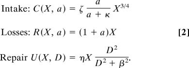The specific functional forms for C and R are analogous to the model of West et al. (27) modified to allow for variable rates of activity. A recent review (28) of the bioenergetics literature supports the mass scalings used here, at least for vertebrates. The dependence of R on activity is true given the definition of a and the dependence of C on activity arises from asserting that encounter rates depend linearly on the energy invested in searching, whereas handling time remains fixed in a Holling type II foraging model. Our choice for the repair function asserts that when damage is low, the energy invested in repair will be near zero and that as damage increases investment in repair will increase until the maximum allocation to repair (η) is reached. In 80% of the cases surveyed, the allocation to repair was <0.5 and >0.9 in only 9%. In preliminary model testing, reducing the exponent from 2 to 1 did not appreciably change the qualitative outcome.

Mortality in this life history model has size- and damage-dependent components. We model the size-dependence of mortality as approximately inversely proportional to length; here a power function of mass with exponent −1/3, with the assumption that size-dependent mortality arises through predation and that activity increases exposure to predators proportionally. This scaling is consistent with several reviews of the size dependence of mortality. For simplicity and based on limited empirical evidence (29), damage-dependent mortality is proportional to the accumulated damage. Thus the rate of mortality is

where μ_a is the rate at which predation risk increases with activity. Note that although Eq. 7 is an equation for mortality, it does not define the shape of the mortality trajectory because neither X(t) nor D(t) are known at the outset. Rather, X(t), D(t), and M(t) are defined by the optimal life history and may a priori take on almost any shape. The model as presented is already nondimensionalized to eliminate redundant parameters. Specifically, we have eliminated proportionality constants for metabolic losses and the size dependence of mortality by rescaling time and size.

We model fitness (F) using lifetime reproductive output given by

where Φ(x, d) is reproductive output per unit time at size x and accumulated damage d. We focus on the evolution of mortality associated with prereproductive growth and activity. Assuming that a switch from growth to reproduction occurs at age T, F may be decomposed as follows

Conditioning F on surviving to age T, we have residual reproductive value

Note that the integral here depends only on mortality subsequent to the growth interval and is clearly a function of size and accumulated damage through their effects on fecundity and mortality after the growth interval. Evaluation of this expression would require dynamical assumptions beyond those already presented. To simplify, we use a product of two power functions to approximate the size and damage dependence of residual reproductive value, i.e.,

where the exponents for size φ_X and damage φ_D are treated as parameters and allowed to range widely.

Working backwards through the growth interval, we define a fitness function F(x, d, t) by

so that F(x, d, t) is the maximum fitness at the end of the growth interval [t, T] taken over activity levels at each instant of time throughout the interval. When t = T, fitness is given by the residual reproductive value, That is, we have (from Eq. 7) F(x, d, T) = V(x, d) = x^φX(1 + d)^−φD.

Fo previous times, F(x, d, t) satisfies an equation of dynamic programming (8–10)

which is solved backwards in time, from t = T − dt to t = 0. Essentially, Eq. 9 works backwards through time calculating present reproductive value by discounting the future reproductive value with the probability of surviving the time interval. The boundaries of the size − damage grid were chosen such that they had no effect on the optimal trajectories for the starting sizes we used. In some of our initial runs, the upper bound for damage was low enough to influence the outcome and mortality plateaus were observed. At t = 0, F(x, d, 0) is the maximum value of F (lifetime reproductive output) attainable given initial size and damage. At each time and state, we generate the optimal level of activity a*(x, d, t), which can then be used to predict growth trajectories by application of Eqs. 1 and 2. For all simulations, we set T = 5 and in general we used dt = 0.05, but setting dt = 0.001 did not change the results.

All of the physiological and life history parameters in the model have mechanistic interpretations and could in principle be determined experimentally (the parameters governing damage, though, may be more difficult to quantify). However, the range of plausible parameter combinations is too broad to investigate completely. So, to analyze the model, we adopted a Monte Carlo approach. We defined ranges for each parameter such that a reasonable amount of growth could occur in the interval [0,T] and that there was some nonzero probability of surviving to the end of the growth interval. We acknowledge that this approach leaves open the question of what happens to mortality trajectories beyond the ranges from which we sampled. However, preliminary sampling outside the ranges reported here did not produce any new trajectory types. For each parameter, this range was divided into up to 30 distinct values (see ref. 12, Table 1) resulting in >10¹⁰ possible parameter combinations. Because this space is too large for complete enumeration, we randomly chose 10,000 parameter sets from these possible combinations and evaluated the optimal life history for each. Parameter sets from this range that produced implausible results (e.g., that the optimal growth trajectory was to never grow) were discarded, leaving ≈3,000 viable parameter sets. The vast majority of nonviable parameter sets resulted in damage accumulation rates that were so costly as to eliminate the feasibility of growth.

To analyze the influence of the different physiological and life history parameters on the resultant mortality trajectories, we used linear and quadratic discriminant functions (30) on the original parameter set and an augmented set that included all pairwise products. Using leave-one-out cross-validation as a model selection criterion, we found that a linear model in the augmented parameter space was optimal and had a cross-validation classification success of 76%.

All of the analyses reported here were carried out by using code written by SM in Matlab v. 6.5 (Mathworks, Natick, MA). This code is available upon request.

References

- 1.Gompertz B. Philos Trans R Soc London. 1825;115:513–583. [Google Scholar]
- 2.Gavrilov LA, Gavrilova NS. The Biology of Life Span: A Quantitative Approach. London: Harwood; 1991. [Google Scholar]
- 3.Wachter KW, Finch CE, editors. Between Zeus and the Salmon: The Biomdemography of Longevity. Washington, DC: Natl Acad Press; 1997. [PubMed] [Google Scholar]
- 4.Carey JR. Annu Rev Ent. 2001;46:79–110. doi: 10.1146/annurev.ento.46.1.79. [DOI] [PubMed] [Google Scholar]
- 5.Carey JR, Judge DS. Population. 2001;13:9–40. [Google Scholar]
- 6.Carey JR. Longevity: The Biology and Demography of Life Span. Princeton: Princeton Univ Press; 2003. [Google Scholar]
- 7.Pearl R, Miner JR. Q Rev Biol. 1935;10:60–79. [Google Scholar]
- 8.Mangel M, Clark CW. Dynamic Modeling in Behavioral Ecology. Princeton: Princeton Univ Press; 1988. [Google Scholar]
- 9.Houston AI, McNamara JM. Models of Adaptive Behavior. Cambridge, UK: Cambridge Univ Press; 1999. [Google Scholar]
- 10.Clark CW, Mangel M. Dynamic State Variable Modeling in Ecology: Methods and Applications. Oxford: Oxford Univ Press; 2000. [Google Scholar]
- 11.Wachter KW. Popul Dev Rev. 2003;29(Suppl):270–291. [PMC free article] [PubMed] [Google Scholar]
- 12.Mangel M, Munch SB. Am Nat. 2005;166:E155–E176. doi: 10.1086/444439. [DOI] [PubMed] [Google Scholar]
- 13.Harman D. J Gerontol. 1956;2:298–300. doi: 10.1093/geronj/11.3.298. [DOI] [PubMed] [Google Scholar]
- 14.Kirkwood TBL, Rose MR. Philos Trans R Soc London B. 1991;332:15–24. doi: 10.1098/rstb.1991.0028. [DOI] [PubMed] [Google Scholar]
- 15.Chu CYC, Lee RD. Theor Popul Biol. 2006;69:193–201. doi: 10.1016/j.tpb.2005.11.004. [DOI] [PMC free article] [PubMed] [Google Scholar]
- 16.Cichon M, Kozlowski J. Evol Ecol Res. 2000;2:857–870. [Google Scholar]
- 17.Mangel M. J Theor Biol. 2001;213:559–571. doi: 10.1006/jtbi.2001.2431. [DOI] [PubMed] [Google Scholar]
- 18.Mangel M. Popul Dev Rev. 2003;29(Suppl):57–70. [Google Scholar]
- 19.Novoseltsev VN, Arking R, Novoseltseva JA, Yashin AI. Evolution (Lawrence, Kans) 2002;56:1136–1149. doi: 10.1111/j.0014-3820.2002.tb01427.x. [DOI] [PubMed] [Google Scholar]
- 20.Yearsley JM, Kyriazakis A, Gordon IJ, Johnston SL, Speakman JR, Tolkamp BJ, Illius AW. J Theor Biol. 2005;235:305–317. doi: 10.1016/j.jtbi.2005.01.009. [DOI] [PubMed] [Google Scholar]
- 21.Mangel M, Bonsall MB. Theor Popul Biol. 2004;65:353–359. doi: 10.1016/j.tpb.2003.07.005. [DOI] [PubMed] [Google Scholar]
- 22.Kirkwood TBL, Holliday R. Proc R Soc London B. 1979;205:531–546. doi: 10.1098/rspb.1979.0083. [DOI] [PubMed] [Google Scholar]
- 23.Drenos F, Kirkwood TBL. Mech Age Dev. 2005;126:99–103. doi: 10.1016/j.mad.2004.09.026. [DOI] [PubMed] [Google Scholar]
- 24.Hamilton WD. J Theor Biol. 1966;12:12–45. doi: 10.1016/0022-5193(66)90184-6. [DOI] [PubMed] [Google Scholar]
- 25.Milne EMG. Mech Ag Dev. 2006;127:290–297. doi: 10.1016/j.mad.2005.11.003. [DOI] [PubMed] [Google Scholar]
- 26.Lander AD. PLoS Biol. 2004;2:0712–0714. doi: 10.1371/journal.pbio.0020164. [DOI] [PMC free article] [PubMed] [Google Scholar]
- 27.West GB, Brown JH, Enquist BJ. Nature. 2001;413:628–631. doi: 10.1038/35098076. [DOI] [PubMed] [Google Scholar]
- 28.Essington TE, Kitchell JF, Walters CJ. Can J Fish Aquat Sci. 2001;58:2129–2138. [Google Scholar]
- 29.Collins AR, Gedik CM, Olmedilla B, Southon S, Beillizzi M. FASEB J. 1998;12:1397–1400. [PubMed] [Google Scholar]
- 30.Hastie T, Tibshirani R, Friedman J. The Elements of Statistical Learning: Data Mining, Inference, and Prediction. Berlin: Springer; 2001. pp. 84–111. [Google Scholar]