Figure 4.

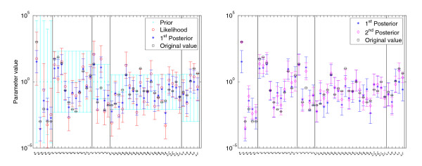
Posterior distributions in the threonine model. Left: prior and kinetics-based posterior in the threonine model. All system kinetic parameters (energy constants $k_i^G$, velocity constants $k_l^V$, k^M and k^I values) and the equilibrium constants $k_i^{eq}$ are listed on the abscissa. Black □: parameter values from the original model. Bars of different colours represent the marginal distributions (mean and standard deviation), corresponding to the arrows in the left diagram. Light blue ●: prior distribution of the logarithmic parameters. Red ○: likelihood function representing artificial experimental values with error bars. Dark blue *: kinetics-based posterior distribution. Right: true values (black □) and first, kinetics-based posterior (blue bars, *). Second, metabolics-based posterior (purple bars, ◇) computed from artificial data. The marginal distributions of kinetics-based and metabolics-based posteriors look quite similar.