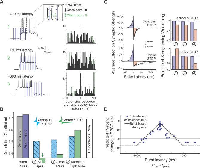
Figure 4. Spike-Timing–Based Rules Must Be Modified to Account for the Observed Plasticity.

(A) Histograms of spike-time latencies (right) measured from the timing between EPSPs and spikes evoked during the three different burst-based stimulation protocols shown (left). Nearest-neighbor times are shown in black, with additional non–nearest-neighbor times in green.

(B) CCs demonstrating the degree to which different learning rules predict the observed data of Figure 3. Spike-based rules from the Xenopus retinotectal system [32] (hashed cyan) and mammalian somatosensory cortex [33] (green)—are compared with the burst-latency–based rules (left columns). Removing consideration of spike pairs that result in weakening produces better predictions: from the naively applied STDP (#1), to only considering nearest-neighbor spikes (#2), to the modified STDP that takes multi-spike interactions into account as suggested by Sjöstrom et al. [34] (#3). Removing the temporal window for depression entirely—leaving a simple spike-based coincidence rule—yields the best predictions (right column).

(C) The ability of spike-based rules to predict the data in (Figure 3) is related to the degree to which depressing latencies are ignored. Left: the average Xenopus (top) and cortex (bottom) learning rule as more spike latencies are selectively ignored. Right: the resulting balance between strengthening (blue +) and weakening (red −) changes with successive modifications to STDP: the best predictions correspond to rules with the least amount of weakening.

(D) The predictions of the spike-based learning rule derived from the total number of spike coincidences, compared with the burst-based rule that is just a function of burst latency (dashed line). t _post, time of the postsynaptic burst; t _pre, time of the presynaptic burst.