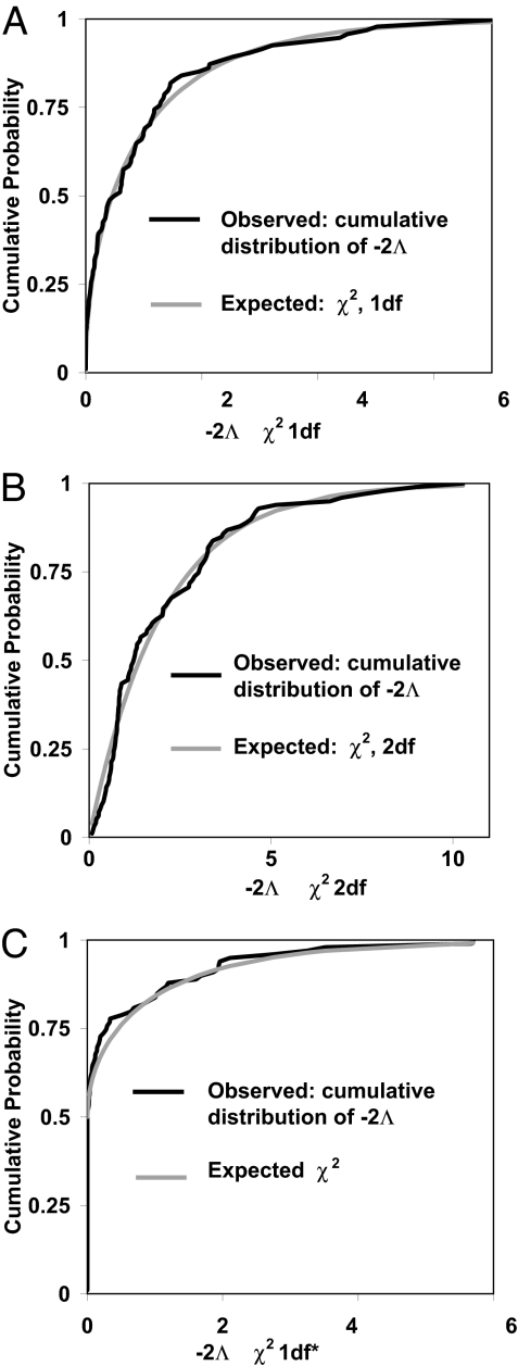
Fig. 2.

Cumulative distributions of −2Λ̂ calculated from Markov chain simulations run on 100 simulated data sets. (A) The true model has two populations of identical size, with simulated data sets sampled following: θ₁ = θ₂ = 10, m₁ = 0.5, m₂ = 0.01, six loci, and 15 gene copies sampled for each population per locus. The MCMC simulation generated 5,000 genealogies with prior maxima: θ₁ = θ₂ = 100, m₁ = m₂ = 5. The observed cumulative distribution of −2Λ̂ is shown with that expected from a χ² distribution with 1 degree of freedom. The Kolmogorov–Smirnov test statistic (the greatest departure between two cumulative distributions), is 0.0851, which does not approach statistical significance. (B) The true model has two populations with identical migration rates and population sizes with simulated data sets sampled following: θ₁ = θ₂ = 20, m₁ = m₂ = 0.1, 25 loci, and six gene copies sampled for each population per locus. The Markov chain simulations generated samples of 8,000 genealogies with prior maximum values as follows: θ₁ = θ₂ = 500, m₁ = m₂ = 1. The Kolmogorov–Smirnov test statistic is 0.0791, which does not approach statistical significance. (C) The true model is an isolation with migration model with unidirectional gene flow. Simulated data sets were sampled following: θ₁ = 20; θ₂ = 40, θ_A = 30, m₁ = 0.15, m₂ = 0, t = 10, 25 loci, and six gene copies sampled for each population per locus. The estimated posterior density has four dimensions [for θ₁, θ₂,θ_A, and m₁ (note that m₂ = 0)]. Given one parameter fixed at the boundary of the parameter space, the likelihood ratio statistic, contrasting the true model and the full five-parameter model, should be asymptotically distributed as a random variable that takes the value 0 with probability 0.5 and takes on a value from a χ₁² distribution with probability 0.5 (23, 37). The Kolmogorov–Smirnov test statistic is 0.0590, which does not approach statistical significance.