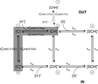
Figure 9. Kinetic model for hPEPT1.

A 7-state model in which the empty carrier is negatively charged (apparent valence −1) and one H⁺ binds to the transporter (C) before the substrate (S). Carrier states at the outer side of the membrane are identified by prime and, at the inner side, by double prime. Details on the transport cycle are given in the Discussion. The partial reaction C₂ ⇌ C₅ represents the H⁺-leak pathway (5% of the transport at saturating substrate concentration). Presteady-state currents are due to the partial reactions C₆ ⇌ C₁ ⇌ C₂, marked by the shaded region. Transitions between conformational states are assumed to be first order or pseudo first order, with rate constants k_ij representing the transition rates from C_i to C_j. Rate constants k₁₂, k₂₁, k₂₃, k₅₄, k₆₅, k₁₆, k₆₁, k₂₇ and k₇₂ are described by voltage-independent values ($K_{\text{ij}}^0$) modulated by voltage and/or ligand concentration, whereas k₃₂, k₃₄, k₄₃, k₅₂ and k₅₆ have a fixed value, and k₂₅ and k₄₅ are obtained by microscopic reversibility (Parent et al. 1992b). The effect of membrane potential (V_m) in k₁₂, k₂₁ k₁₆ and k₆₁ is assumed to follow the Eyring rate theory with symmetric energy barriers (Parent et al. 1992b). α and δ are the fractional dielectric distance coefficients at α = 0.27 and δ = 0.73 (Mackenzie et al. 1996a). The voltage dependence of C₂ ⇌ C₇ is defined by the empirical coefficient 0.37. μ is the electrochemical potential FV_m/RT. To simulate the presteady-state currents in the absence of substrate and the characteristics of Gly-Sar transport, the following set of parameters was used: $K_{12}^0$ = 1.5 × 10⁸ m⁻¹ s⁻¹, $K_{21}^0$ = 550 s⁻¹, $K_{23}^0$ = 10⁵ m⁻¹ s⁻¹, $K_{32}$ = 200 s⁻¹, $K_{43}$ = 600 s⁻¹, $K_{45}$ = 2000 s⁻¹, $K_{54}^0$ = 10⁵ m⁻¹ s⁻¹, $K_{56}$ = 500 s⁻¹, $K_{65}^0$ = 1.5 × 10⁸ m⁻¹ s⁻¹, $K_{61}^0$ = 35 s⁻¹, $K_{16}^0$ = 310 s⁻¹, $K_{25}$ = 1 s⁻¹, $K_{52}$ = 10⁻¹ s⁻¹, $K_{27}^0$ = 5 × 10⁵ m⁻¹ s⁻¹ and $K_{72}^0$ = 800 s⁻¹. The characteristics of cefadroxil transport were simulated by changing $K_{23}^0$, $K_{32}$, $K_{45}$, $K_{54}^0$ and $K_{27}^0$ to 1.25 × 10⁴m⁻¹ s⁻¹, 25 s⁻¹, 250 s⁻¹, 1.25 × 10⁴m⁻¹ s⁻¹ and 3 × 10⁶m⁻¹ s⁻¹, respectively. The total number of transporters, estimated from Q_max (Loo et al. 1993), was 7 × 10¹⁰, and the temperature was 20°C. The predictions of the model are shown by the curves in Figs 5–7, and given in Tables 1 and 2.