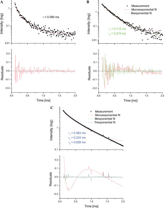
Figure 6.

The exponential decay fitting process used in the study. The exponential decay data were fitted with mono, bi- or tri-exponential decay curves. An example of the best fit in each category (1, 2 or 3 lifetimes) was presented. (A) WT construct at pH 5.6 best fitted to one-lifetime decay. τ ≈ 0.09 ms. (B) Construct ΔU74 at pH 7.2 best fit to two-lifetime exponential decay. τ₁ ≈ 0.12 ms; τ₂ ≈ 0.27 ms. (C) Construct WT at pH 7.2 best fitted to three-lifetime exponential decay. τ₁ ≈ 0.06 ms; τ₂ ≈ 0.22 ms; τ₃ ≈ 0.63 ms. The residuals represented the differences between experimental data and fitting curves, which showed the goodness of fit. The choice of the number of lifetimes is based on the R² and χ² values. The improvement of the fit was shown by comparing other fits and the residue figures. Residuals refer to the difference between theoretical and experimental data.