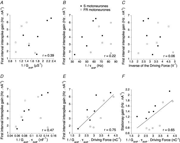
Figure 1. Correlations between the gain and the parameters of the AHP.

In all plots, the filled circles correspond to the 6 motoneurones classified as S type and the open squares to the 6 motoneurons classified as FR types. The gain for the first interspike interval is plotted against the inverse of the AHP conductance (A), the inverse of the AHP decay time constant (B), and the inverse of the AHP driving force (C). The driving force is the spike voltage threshold minus the reversal potential. The criterion used for determining the spike threshold was that the voltage derivative reached 10 mV ms⁻¹ (Brownstone et al. 1992; Sekerli et al. 2004). D, gain for the first interspike interval against the inverse of the product of the AHP conductance and the decay time constant. E, gain for the first interspike interval against the inverse of the product of the AHP conductance, the decay time constant and the driving force. The continuous line is the best linear fit computed with the least squares method. F, stationary gain against the inverse of the product of the AHP conductance, the decay time constant and the driving force. The continuous line is the best linear fit. The coefficient of correlation is given in each panel.