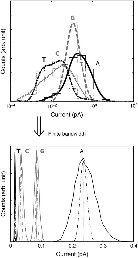
FIGURE 3.
Top graph shows the probability distributions, assuming instantaneous measurements, of currents at a bias of 0.1 V for poly(X)15, where X is A/T/C/G for the solid black, dash-dotted black, dotted gray, dashed gray curves, respectively. The thin lines show the actual current intervals used for the count, whereas the thick lines are an interpolation. After the driving electric field is turned off, the system is left to equilibrate for 200 ps before samples are taken. Each distribution is made up of 1200 samples, each taken with a 1-ps interval. The bottom graph again shows the probability distributions, but now with the assumption that each measurement is time averaged in between each sample. The solid/dashed-dotted line assumes that the distributions in the top graphs are sampled 100/1000/107 times for each new data point.

