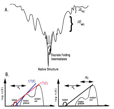
Figure 1.

(A) Schematic diagrams of a protein’s energy landscape and energetic distribution of its density of states. The landscape is characterized by the protein’s energy and entropy. The top of the funnel depicts the large ensemble of random coil configurations. As the energy decreases so does the number of configurations until the lowest energy state is reached, which is the protein’s unique native structure. (B) The density of states histograms show the same picture but emphasize the relationships between the characteristic temperatures (T_f, T_c and T_g) and δE_s, δE_c, and ΔE. They depict two possible folding scenarios. (Left) An energy landscape in which the protein will first collapse upon cooling and then fold. (Right) A case that will lead to faster folding for the stability gap is large enough that the kinetically relevant ruggedness at the transition state will be smaller and folding will occur directly from a random coil. Because we want to optimize against even the worst folders, we will use the scenario at left for our optimization procedure.