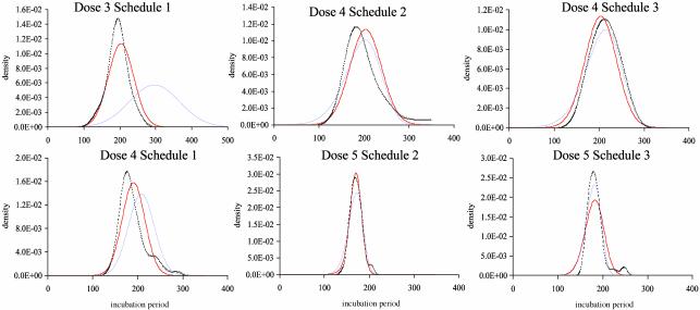
Fig. 4.
IP models. Observed IP at each dose/schedule combination is given by the dotted line (kernel density estimate by using s-plus software, Insightful, Seattle). The fit of the independence model is given in blue, and the alternative model is in red. Estimated distributions [N(μi, σi)] for the independence model at dose levels 3, 4, and 5 are N (296, 70), N (208, 29), and N (164, 10), respectively. For the alternative model, the distributions for doses 3, 4, and 5 in schedule 1 are N (204, 35), N (191, 25), and N (164, 10). The deviation from independence is quantified by the parameters δj1,..., δj9. For schedule 2, the parameters are, respectively, 301, 298, 296, 294, 292, 290, 289, 287, and 286 at dose 4 (σ = 34) and –18, 376, 265, 1,150, 367, 99, 98, 101, and 96 at dose 5 (σ = 13). For schedule 3, the parameters are 330 for all δ at dose 4 (σ = 28) and 7, 148, 410, 722, 1,027, 1,285, 1,471, 1,580, and 1,618 at dose 5 (σ = 24). Log-likelihoods are –1,256 (model 10) and –1,208 (model 11).

